10 Excel Tips to Increase Productivity
In this guide, we’re going to show you 10 tips to increase your Excel productivity for when working with spreadsheets.
Tip 1: Cell styles
You can change the color, font type and borders around cells. Modifying these elements can help distinguish specific cells from others. A good example is changing he coloring of inputs and outputs. If you give different colors to inputs and outputs, users will be able to easily identify cells they need to interact with.
Below is an example of a spreadsheet with and without styling.

Streamlining your formatting tasks in Excel doesn't require starting from scratch each time. Unleash the power of Excel presets to effortlessly apply consistent colors and fonts to selected cells.
Navigate to the Cell Styles section conveniently located under the Home tab on the Ribbon. Simply click the small arrow to unveil a range of options tailored to meet your formatting needs. This efficient approach not only saves time but also ensures a cohesive and polished look across your Excel sheets. Enhance your productivity with these quick and accessible formatting tools.

Choose from a variety of styles to instantly elevate the visual appeal of your Excel spreadsheet. For those seeking a more personalized touch, simply click on the New Cell Style button located at the bottom of this section to craft your own unique style. Once created, custom styles will be conveniently listed in this section for easy access.
Now, let's delve into another insightful styling tip that not only enhances the aesthetics but also boosts your overall Excel productivity.
Tip 2: Sheet Coloring
Another way to increase your productivity in Excel is by changing the color of the sheets tab. If your workbook has a multiple sheets, coloring them is a good example for easing navigation.
All you need to is right-click on a tab and select a color from the Tab Color pane.

Tip 3: Filtering & Sorting
If you are keeping data in tabular form, use Excel’s Filter and Sort features to access what you need faster.
Although either feature can be accessed through the Data tab in the Ribbon. Just right-click on a cell under the column you want to filter or sort.

You can find more information on Sort and Filter features in the following articles:
The crux of organizing your data: How to sort in Excel
How to Filter a Table in Excel
Our next tip involves using named ranges.
Tip 4: Excel Efficiency with Named Ranges
In the realm of Excel functionality, named ranges serve as indispensable tools, allowing users to assign friendly names to specific data ranges. These user-defined names not only streamline the writing of formulas but also enhance readability. Consider the following example:
With names: =SUMIFS(HP,Generation,"I",Type,"FIRE")
The clarity introduced by named ranges is evident - no longer must one recall which range corresponds to specific data. By incorporating names into your ranges, formulas become more intuitive and easier to manage.
Adding names to your ranges is a straightforward process. Simply select the desired cell range and enter the name into the reference box, located just before the formula box on the top bar. This simple yet powerful practice not only enhances your Excel workflow but also contributes to a more organized and efficient spreadsheet experience.

There is a naming convention you need to obey while assigning names into the ranges. Check our Excel Named Ranges Guide to learn more and find examples.
Tip 5: Tables
Tables is an Excel feature which can be used to format, manage, and analyze your data. By converting your regular range of cells into a table, your data gains a dynamic formatting and special reference system which makes formula auditing process easier like named ranges.

You can convert your data in tabular layout into an Excel Table easily by selecting a cell in the data and pressing Ctrl + T. For more and detailed information, please check the following articles:
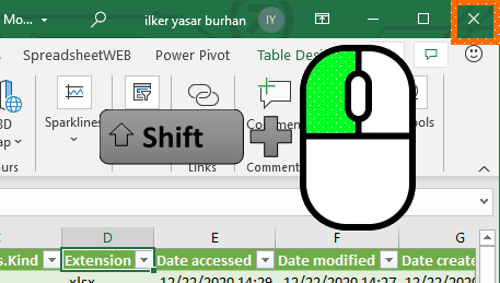
Tip 6: Keyboard and Mouse Shortcuts
Optimize your Excel workflow with efficient combinations of keyboard keys and mouse buttons to streamline tasks effortlessly. Enhance your productivity by utilizing time-saving shortcuts – for instance, the F4 key allows you to conveniently repeat your last action. Moreover, expedite the process of closing multiple Excel windows by holding down the Shift key while clicking the Close (X) button. Discover these valuable tips to boost your efficiency and make the most out of your Excel experience.
Find more about useful Excel shortcuts from below pages.
10 Most Useful Shortcuts in Excel
Tip 7: Incremental Tab Names
If your sheet names include or end with incremental numbers like 2020, 2021, 2022 or Year 2020, Year 2021, Year 2022, putting the numeric value inside parenthesis () will increase the number when you copy the sheet.

Tip 8: AutoSave / OneDrive / Threaded Comments
If you are a Microsoft 365, also known as Office 365, subscriber, you will see the AutoSave switch at the top left of your Excel menu.

Turn this switch on to enable AutoSave feature which constantly saves your worksheet into your OneDrive account. The obvious benefit is eliminating the data loss. Other significant advantage is that it gives you ability to share your workbook with others easily. Anyone you give the permission can work on the workbook at the same time.
You can leave threaded Comments to anyone using the workbook as well.

Tip 9: Send as attachment
If you send your Excel workbook or a part of it as an email attachment occasionally, this tip may save you lots of time. You can send your workbook as an email attachment with a few clicks.
The native way is to use the Share function in the File menu. Click the Share button in the File menu to display Share dialog where you can find attach options. Each button attaches your workbook into an email.

Another way to access these options is to add the commands into your Quick Access Toolbar. Both functions as well as E-mail as XPS Attachment command can be added In Excel Options > Quick Access Toolbar dialog.

You can find more commands to increase your productivity in Hidden commands in Excel.
Tip 10: Pivot Tables
With Pivot Tables, grouping and consolidating data can be done quickly with a few drag & drop actions.

You can learn about Pivot Tables here: How to Organize and Analyze Your Data Quickly with Excel’s PivotTables guide. Also, don't forget to check the Microsoft's official website for further reading!