Introduction to Basic Excel Financial Formulas
In this article, we delve into the essential formulas that serve as the backbone for financial modeling and calculations in Excel. Whether you are a beginner aiming to establish a solid foundation or an experienced user seeking to refine your financial skills, this guide provides a comprehensive understanding of the basic Excel financial formulas integral to effective financial planning and analysis for your personal finances.
SUM Function in Financial Formulas
Instead of selecting individual cells and entering the ‘+’ in between, use the SUM function to add up an entire range of values, especially when working with excel financial formulas. When managing your personal finances, there are two compelling reasons why you should opt for the SUM function over the regular addition operator (+).
The first notable advantage of the SUM function is its efficiency in handling multiple cells. You can effortlessly select all adjacent cells at once, and the SUM function will automatically add up all values within that range, streamlining the calculation process.
Moreover, the SUM function excels in financial scenarios by adding only numerical values, thereby avoiding any errors related to non-numeric entries. Utilizing the plus sign (+) for addition in financial formulas may result in a #VALUE! error, whereas the SUM function ensures precision in summing up relevant numeric data.
In summary, when working on financial calculations in Excel, incorporating the SUM function not only enhances efficiency by allowing you to select entire ranges but also guarantees accurate results by excluding non-numeric values from the calculation process.

Using SUBTOTAL
The SUBTOTAL function in Excel is a versatile tool, acting like a Swiss Army Knife by performing functions ranging from calculating averages to finding variances. By assigning a number from 1 to 11 as its first argument, it adapts its purpose accordingly. We specifically use 9 for SUM functionality. What sets SUBTOTAL apart is its ability to avoid interfering with other SUBTOTAL functions during calculations, making it ideal for displaying subtotals.
In the realm of excel financial formulas, the SUBTOTAL function, when used with the format =SUBTOTAL(function_num, ref1, [ref2], ...), proves invaluable. Incorporating the keyword "excel financial formulas" emphasizes its significance in financial calculations, especially when summing values evenly distributed. This function becomes a dynamic tool for precision in crafting comprehensive financial models and analyses.
Let's see how this works on an example.

In the realm of financial data analysis, Excel proves to be an invaluable tool. The cell D7 in our financial spreadsheet contains a SUBTOTAL function equipped with the SUM (9) ability, targeting the range D8:D19 for summation. However, an interesting challenge arises—within this range, we already have two sets of totals positioned at rows 8 and 15. In standard situations, this could result in a double-counting dilemma. This is where the prowess of Excel financial formulas comes into play.
Despite the presence of subtotal values in cells D8 and D15, the SUBTOTAL function in D7 comes to the rescue. By strategically incorporating the SUBTOTAL function in both of those cells, we ensure that the totals are not counted multiple times. In essence, the SUBTOTAL in D7 intelligently avoids duplicating calculations performed by SUBTOTALS in D8 and D15. This nuanced approach, empowered by Excel financial formulas, streamlines the accuracy of our financial analysis and ensures meticulous handling of data, a crucial aspect in financial modeling and reporting.
Using VLOOKUP
The famous VLOOKUP formula, a key component in Excel financial formulas, can efficiently and vertically look up data within tables. This formula becomes particularly valuable when dynamically calculating budgeting tools, ensuring that you won't have to worry about formatting or other functions.
In the context of Excel financial formulas, the VLOOKUP utilizes the first column of your financial data to search for the specified lookup value. Once it locates the lookup value in a row, the formula returns the value specified in the column number within the table array. The very last parameter of the formula is crucial, as it determines whether the lookup should be exact or approximate (range lookup).
=VLOOKUP(Lookup_value, table_array, col_index_num, [range_lookup])
For example, begin by creating a list of your items and their base amounts.

Make a drop-down list by selecting the entire list and go to Data Validation.

Finally use the VLOOKUP function for monthly costs.

Before copying your formula to other months, make sure that the search column of the first argument and the whole data range are absolute references. The dollar sign ($) indicates that a row or column reference that comes before it is absolute. For instance, $B24 means column B is absolute, but row number is still relative (will be updated when copied).
For more detailed information see, HOW-TO VLOOKUP
AutoSum in Financial Formulas
The AutoSum is not a function but a useful feature found under the FORMULAS ribbon in Excel that can significantly expedite the creation of budgeting applications. This AutoSum menu provides quick access to essential operations such as sum, average, count, maximum, or minimum of a set of values. Incorporating Excel financial formulas becomes even more efficient with the AutoSum feature, streamlining tasks related to budget calculations and distribution. This can be especially beneficial for those looking to enhance the speed and accuracy of financial computations in Excel.

Selecting one of these options will insert the corresponding function into the selected cell. AutoSum is a smart feature as it can predict the range you want to use in the function, and automatically place the function you choose.
Begin by selecting your data and then make your selection or press the shortcut for that action. For example, you can press Alt + = to add SUM functions below your data. Alternatively, you can choose any function you want under menu option.