A subtotal is the aggregation of a data set, typically showing the totals of a certain section in that data set. A budgeting spreadsheet is a good example for this where subtotals are used to display more details of certain categories. In a budgeting application, you may want to categorize the expenses, and break them down like household, transportation, and social activities. In this guide, we're going to show you how to calculate subtotal in Excel.
Using generic functions
The subtotal calculations are basic aggregation operations. You can easily get the subtotals using functions like SUM, AVERAGE or COUNT. On the other hand, using these formulas in the middle of tables can sometimes cause issues. Especially, when you need to get total of every section. In this case, you either need to use other formulas to ignore those subtotal values, or set ranges individually for each formula to avoid calculating those values multiple times.
In the example below, the SUM function is used to calculate the total of each Home Expenses and Transportation, as well as a grand total. Although the total expense value should be 655 (455 + 200), the formula in cell F28 shows 1,310. The reason is that the SUM function calculates the subtotal values with the actual data.

This can be resolved by excluding the subtotal cells from the function. or subtracting them from the result. However, this obviously means additional work initially, and when you need to update your table. Excel's solution to these types of scenarios is the SUBTOTAL Function.
Using the SUBTOTAL Function to calculate subtotals in Excel
The SUBTOTAL function is like the Swiss Army Knife of Excel functions. The function combines several capabilities in a single function, and also has two additional features:
- Ability to ignore other SUBTOTAL functions in the range
- Exclude filtered and hidden rows from the calculation
These two features make the SUBTOTAL function a perfect tool to calculate subtotals in Excel (obviously!). Let's see how you can use the function.
The SUBTOTAL function can replicate what other functions does. Supported functions include:
| 1. AVERAGE | 2. COUNT | 3. COUNTA |
| 4. MAX | 5. MIN | 6. PRODUCT |
| 7. STDEV | 8. STDEVP | 9. SUM |
| 10. VAR | 11. VARP |
To define which function you want to replicate, you need to enter its defined code as an argument. After this, enter the other arguments as if you were using that function. For example, use 9 for a sum operation.
If the aggregation range doesn't contain any other SUBTOTAL functions, both formulas return the same result.

Calculating the subtotal in Excel
Where the SUBTOTAL function shines is when you need to calculate all values. If you are using the SUBTOTAL, you do not need to worry about duplicate calculations. The function ignores its counterparts in the selected range. Thus, you will get the sum of all data without issues.
The example below shows how the SUBTOTAL and the SUM functions work in unison. While the SUBTOTAL returns the correct value (655), SUM returns double that value (1310).

Ignoring filtered and hidden rows
Another benefit of the SUBTOTAL function is its ability to ignore hidden rows and columns when aggregating the data. By default, the function ignores all values that are filtered out . On the other hand, you need to change the code of operations to enable this.
Instead of using codes from 1 to 11, use the numbers between 101 and 111 in the respective order. For example, 101 for COUNT instead of 1, 102 instead of 2, and so on.
You can see the difference in the example below. The formulas on the left side do not ignore the hidden rows between 9 and 11. These 3 rows have total of 110. As a result, while the left side shows 455 as total value, the formula on the right side shows 345. The difference is 110.

For more information and examples, please see: SUBTOTAL.