Comparing the data in two different columns is a frequently used method in data analysis. In Excel, you can compare using formulas or highlighting. In this guide, we’re going to show you how to compare two columns in Excel using these two methods.

Compare two columns in Excel using formulas

For a row-by-row comparison, you need to use an IF function for comparing two cells in a row, and then return a value indicating the result. Type in the formula in an adjacent column in the same row as your data, and then copy it down all the way for the rest of the rows you'd like to compare.

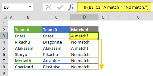
A comparison using the equal sign (=) will not be case-sensitive. If you need to compare for exact values, use the EXACT function. The EXACT function compares two values and returns a Boolean value, which can be used for the logical test in an IF function.

Compare two columns in Excel using highlighting

Using the highlighting method can help distinguish the outliers better. With this method, you can color (highlight) cells dynamically using the Conditional Formatting feature. Here are the steps:

1. 1. Select both columns to be compared.
   2. Open the Conditional Formatting window by going to HOME > Conditional Formatting > Add New Rule.
   3. Select Use a formula to determine which cells to format item.
      
   4. Enter a comparison formula that includes absolute column references (=$B3=$C3). Use the Format button to open Format Cells dialog and chose a background (fill) color.
      
   5. Click OK to continue and apply your settings.
      

Compare two columns in Excel entirely using formulas

If you want to compare two columns regardless of how many times they match, you need to use same approach as shown in "using formulas" section, but using different formulas. The COUNTIF function counts the number of occurrences of a specified value in a range, and returns the count. We can use the outcome of this function to verify if a value from one column also exists in the other. If the result of the COUNTIF formula is greater than 0, it means that the value exists in both columns.

Enter the formula in an adjacent column in the same row, and copy it down for all columns to be compared. Alternatively, you can use the COUNTIFS function, which can work with a cell range.

Compare two columns in Excel entirely using highlighting

Highlighting matched cells requires adding two rules in order to compare two columns for any number of matches. The formula syntax remains same for this approach, but you need to adjust the formulas for both columns. Below are the formulas based on our example:

While the formula for the column B is looking for $B3 in $C$3:$C$8, the formula for the column C is looking for $C3 in $B$3:$B$8.