Conditional Formatting is commonly used to highlight data fields to easily identify outliers, or narrow down the results. However, this feature works a bit differently when dealing with a Pivot Table. Pivot Tables are also dynamic elements, and conditional formatting rules won't apply when the table size changes. In this guide, we’re going to show you how to use conditional formatting Pivot Tables.
Begin by selecting any value from your able. You do not need to select the entire range like when applying conditional formatting.

Go to HOME > Conditional Formatting > New Rule to add a new formatting rule, or select from predefined options. If you select the latter, you will need to configure the rule regardless.

The New (or Edit) Formatting Rule window contains options specific to Pivot Tables. You can choose the location where you want to apply your conditional formatting rule. Let's look on the options:

Selected Cells
The Selected Cells option, as the name suggests, only applies conditional formatting to the selected cells. The rule won't not update its range when the Pivot Table is modified. We don't recommend using this option unless you are sure that the Pivot Table size will remain static.

All cells showing "Sum of Total" values
This option includes all cells under the Sum of Total column. If you are not familiar with Pivot Tables, Sum of Total is the name for a column that contains the aggregated values of the column Total. As a result, you will see a different wording in this option. Use this option to apply conditional formatting rule to all cells under the column of the selected cell. The range of the conditional formatting rule will be updated with the Pivot Table.

All cells showing "Sum of Total" values for "Type"
This option adds a criteria to the second option. The conditional formatting rule will be applied to the Sum of Total values of Type rows only. Similar to the second option, Type is a column specific to our data. Choose this option to apply formatting only to the specific values in the Pivot Table. You can see that the Generation and Name rows are not affected by conditional formatting.

For more information about conditional formatting, please see how to highlight.