What is Excel Power Pivot?
Welcome to our easy-to-follow guide on Excel Power Pivot! This guide is perfect for anyone who wants to make the most out of Excel for business intelligence and data analysis. Power Pivot is an incredible tool in Excel that helps you work with big data sets and create detailed data models. It's fantastic for importing data from various sources, doing complex calculations with DAX (Data Analysis Expressions), and making interactive reports and dashboards. First of all, let's have a look at what DAX is;
DAX is like a set of advanced formulas in Excel, designed to work with data models. It's not just about simple calculations; DAX helps you to perform complex data analysis and create sophisticated data models. This makes it a must-know for anyone looking to dive deeper into business intelligence and advanced data analysis in Excel.
Key Features of DAX
-
Easy to Learn for Excel Users: If you're familiar with Excel formulas, you'll find DAX understandable. It's designed to be intuitive for those who have basic knowledge of Excel functions.
-
Powerful Data Analysis: DAX goes beyond basic calculations. It can handle complex data analysis tasks, making it perfect for creating detailed reports and dashboards in Excel Power Pivot and Power BI.
-
Dynamic Calculations: With DAX, your data calculations can become more dynamic and responsive to changes in your data, providing more in-depth insights.
-
Enhancing Power Pivot and Power BI: DAX is essential for making the most of Excel's Power Pivot and Power BI, allowing you to create robust data models and analytics.
Getting Started with DAX
- Start with Basic Functions: Begin by learning the basic functions and gradually move to more complex ones. This will help you build a strong foundation.
- Practice with Real Data: The best way to learn DAX is by applying it to real-world data scenarios in Excel.
In this tutorial, we'll break down what Power Pivot is, how it functions, and how you can use it to draw important insights from your data. This tool is a game-changer whether you're a business analyst, a data expert, or just love Excel. Let's explore the amazing capabilities of Excel Power Pivot and see how it can change the way you work with data.
Microsoft has developed a range of "Power" tools for Excel, like PowerQuery and PowerBI. PowerPivot is one of the first in this series, and it's incredibly powerful, even if it's not as well-known.
With Power Pivot, you can easily handle millions of data rows, quickly analyze information by linking different types of data, and create calculated columns and measures using formulas. Sounds interesting? Let's dive in.
While you can do a lot of things directly in Excel, PowerPivot saves you time and can handle more complex tasks. It works with SQL Server Analysis Services (SSAS) to crunch numbers fast, and offers cool data analysis tools like Power View, Power Map, and Excel's standard features. Plus, PowerPivot works smoothly with DAX for data manipulation, giving you fast results no matter how large your file is.
Join us as we make Excel Power Pivot simple and show you how to use this powerful feature to enhance your data analysis skills.
Key Features of Excel Power Pivot:
- Handling Large Data Sets: Power Pivot is designed to work efficiently with large data sets that traditional Excel sheets might struggle to process. It can handle millions of rows of data, providing the horsepower needed for heavy data analysis tasks.
- Advanced Data Modeling: With Excel Power Pivot, you can create sophisticated data models. This includes building relationships between different data tables, creating calculated columns and measures using DAX (Data Analysis Expressions), and transforming raw data into meaningful information.
- Seamless Data Integration: Power Pivot allows the integration of data from various sources. Whether it's SQL databases, data feeds, or other spreadsheets, it can bring together disparate data sources into a single comprehensive analysis tool in Excel.
- Enhanced PivotTable Capabilities: Power Pivot supercharges PivotTables in Excel, offering advanced features like creating calculated fields, using slicers to filter data, and the ability to process large amounts of data without slowing down your workbook.
- Dynamic Reporting and Business Intelligence: It enables the creation of dynamic reports and dashboards. This feature is crucial for business intelligence, helping in the visualization and analysis of business data for strategic decision-making.
Utilizing Excel Power Pivot for Optimal Data Analysis:
- Data Analysts and Business Professionals: Excel Power Pivot is a must-have tool for data analysts and business professionals who require advanced data processing and analysis capabilities in Excel.
- Interactive Data Exploration: Use Power Pivot to explore and analyze your data interactively. Its powerful features allow for deep dives into data and uncovering insights that might be missed in traditional spreadsheets.
- Customized Reporting: Create customized reports and dashboards tailored to your specific business needs. Power Pivot provides flexibility and power in presenting data that speaks directly to stakeholders.
Getting Started to
PowerPivot is available as a free add-in for Excel 2010 and is included natively in Excel 2013 and later. Excel 2010 users will need to download and install the free add-in from Microsoft’s website. Once installed, the PowerPivot ribbon will appear in the top menu. Power-Pivot add-in download
Excel 2013 and Excel 2016 users simply need to enable it from add-in options. To do this,
- Go to File > Options > Add-Ins.
- Under the Manage box, click COM Add-ins and press Go.
- Make sure the Microsoft Office Power Pivot box is checked and click OK. If you have other versions of PowerPivot installed, those versions will also be listed in the COM Add-ins list. Make sure you select the PowerPivot add-in for Excel.
What You'll Learn with This Guide:
-
Understanding Data Models: We'll start by explaining what data models are and why they're crucial in data analysis. In simple terms, a data model is a way to organize and connect different pieces of data to draw meaningful insights.
-
Getting Started with Power Pivot: Even if you're new to Power Pivot, our guide will make it easy to understand. We'll walk you through the basics of how to activate and navigate Power Pivot in Excel.
-
Importing and Integrating Data: Learn how to bring data into Power Pivot from various sources. Whether it's Excel sheets, databases, or other data files, Power Pivot makes it easy to compile everything in one place.
-
Creating Relationships Between Data: One of the key strengths of Power Pivot is its ability to link different data sets together. We'll show you how to create these relationships, which are essential for building a comprehensive data model.
-
Enhancing Data with Calculations: Discover how to use DAX (Data Analysis Expressions) to add calculated columns and measures, giving more depth and functionality to your data model.
-
Visualizing Data: Finally, we'll explore how to use your data model to create impactful reports and visualizations directly in Excel.
Excel Power Pivot: Creating a Data Model
PowerPivot offers various options to import data into a data model. Let’s see how this works with an example. Here, we have two tables, one table contains a breakdown of finances by state, and the other matches state names with their abbreviations. You can download these workbooks here and here.

Let’s begin with starting the add-in. You can do this by clicking the Manage button under the PowerPivot menu.

The PowerPivot for Excel window serves as the control center for managing your data connections and the intricate relationships between tables, making it a crucial component in building a comprehensive data model. This functionality is key to leveraging PowerPivot's robust capabilities in Excel.
When you open the PowerPivot window, you'll be greeted with a range of options for importing and connecting to various data sources. These sources include powerful databases and simpler file types, ensuring flexibility and ease in how you gather and manipulate data. Some of the notable connection options you'll find include:
- Microsoft SQL Server: Ideal for those working with large, enterprise-level databases. PowerPivot can directly tap into SQL Server databases, allowing you to pull data right into your Excel environment.
- Microsoft Access: A good option for those who manage their data in Access databases. Importing data from Access into PowerPivot is straightforward and efficient.
- Oracle: For users dealing with Oracle databases, PowerPivot provides a seamless connection, enabling the integration of complex data sets into your Excel model.
- Data Feeds: These are perfect for importing data from web services or other data feed sources. PowerPivot can connect to various data feeds, making external data integration hassle-free.
- Excel or Text Files: If your data is stored in Excel sheets or simple text files like CSV, PowerPivot can easily import this data. This is particularly useful for combining and analyzing data from multiple Excel files or importing data from legacy systems that export to text files.
In this example, our focus will be on connecting PowerPivot to an Excel file. This is a common scenario for many users who are looking to enhance their existing Excel data with the powerful features of PowerPivot.
To start the process, you'll need to click on the "From Other Sources" button. This action will open a new window, where you can view all the available connection options. Here, you'll see a list of data sources that PowerPivot can connect to, along with detailed instructions on how to establish these connections.
Once you select the option to connect to an Excel file, you'll be guided through a series of steps to locate and import your data. PowerPivot handles the import process efficiently, allowing you to quickly integrate your Excel data into the PowerPivot environment where you can begin your advanced data analysis.

Next, select the data source you’d like to connect to. We’re going to pull data from an Excel file, so select Excel File to proceed.

Click Browse to locate your source file. If your data includes column headers in the first row of your data file, make sure the Use first row as column headers is checked.

Click the check boxes next to the table (sheet) names to add them to the data model. We have two tables here, first for financial numbers which has the state abbreviations, and second one with full state names and abbreviations. If you connect to a relational database and your tables have relationships with other tables, remember to press the Select Related Tables button and this way the system will catch all necessary tables.

When you’re done, press Finish and wait for Excel to do its magic. Click Close to end the process and import the data into your spreadsheet.

Our data model is ready. You will see that the PowerPivot for Excel window is now filled with imported data. These tabs represent data tables and they behave differently than workbook sheets. At this point, you can manipulate the tables, refresh data or even create Pivot Tables or Pivot Charts.

Calculated Fields
PowerPivot also allows you to add calculated fields into your table. This is a pretty useful way to manipulate big sets of data. While calculated fields compute values row by row, measures aggregate values. To add calculated fields, you need to use Data Analysis Expressions (DAX). DAX is very similar to Excel formula, but are more suited for data analysis tasks. To create a calculated column follow these steps,
- Press Design in the toolbar and click Add under the Column

- Type in your formula. For example,
=IF([End Of Year Assets]>=[Average Assets],"Good","Bad")

- Rename the column by right clicking, and selecting Rename Column. Here, we changed the column name to “Status”.

- The new column will be added to the right of your table.
Relationships
Now let’s see how we can create relationships between tables. As our example goes, the main table contains the financial data and state abbreviations, and other one has full names. To match the two files and have our main table display state names instead of the abbreviations, we can establish relationships between the two.
Note: You might be asking yourself, why not just put everything together in a simpler way, like using formulas. However; if you have 10 tables, or billions of rows (or even worse both), every column will have a serious performance impact on calculations. This concept is called Data redundancy. To learn more, https://en.wikipedia.org/wiki/Data_redundancy
Begin by clicking Diagram View icon in the toolbar.
 Here, you can manage relationship between tables, hierarchies and KPIs.
Next, we need to drag and drop the related fields into corresponding sections. Please note that the relationship direction should be either from one occurrence to one occurrence, or from many occurrences to many occurrences. In other words, many to one relations won’t work. If there are more than one instance for a value, you might get errors.
For example, in the Breakdown table some state names are used more than once, while in the States table we see a state name only once. This is in accordance with the relationship direction as it needs to be from State in Breakdown table to Abbreviation in the States table.

Next, let’s see how we can create visualizations from this table. Begin by clicking Pivot Table in the toolbar and create a Pivot Table, or click the arrow to see more options. In our example, we selected Chart and Table (Horizontal), but feel free to experiment.

We start from the Pivot Table to show how relationship works. From PivotTable Fields on the right hand side, move the State field from the States table, into the ROWS section. Then move the End of Year Assets in the Breakdown table, to VALUES section. Now we should have the full state names and our data on a table. To learn more about pivot tables and how awesome they are, see our How to Organize and Analyze Your Data Quickly with Excel’s PivotTables guide to learn more.

Pivot Charts work very similar to Pivot Tables. Simply drag and drop the data fields into AXIS (CATEGORY) sections and statistical fields into VALUES section.

Relationship Between Pivot Charts and Pivot Tables
Pivot Charts and Pivot Tables in Excel are both great for understanding and working with lots of data. They share a few key features that make them really useful for anyone using Excel. Both of them let you arrange and summarize big data sets in a way that's easy to get. You can change how you view your data in both Pivot Tables and Pivot Charts, which helps you see your data in different ways. They are connected to the same data, so if you change something in your data, both the chart and the table will update. This makes analyzing data in Excel much simpler, as you can see changes immediately. For anyone dealing with lots of numbers - like business analysts or data scientists - using Pivot Tables and Pivot Charts together is a great way to make sense of all that information and make good decisions. They are really helpful for showing your data in a clear and helpful way.
PowerPivot is a hidden gem that is not known to all Excel users. It’s a very powerful tool that can handle a vast amount of data, while allowing you to manage connections and manipulate the data. It sure can make life much easier when dealing with data tables and their analysis. Dive into Excel Power Pivot to explore its full potential in transforming your data analysis process. Harness its power to make more informed decisions, understand complex data scenarios, and present your findings in compelling, insightful ways.