Do you need only dates in a certain field? No problem, just set the data validation options to enforce that. Need more detailed restrictions that can only be defined with a long formula? Enter data validation – Excel doing your data cleaning for you by preventing data entry errors before they happen. You won’t believe how much time this approach will save you when it’s time to organize your tables.
Data validation is also the key to creating dropdown-style inputs, where the input will only accept entries from a predetermined list of items. Let’s take a look at how you can utilize this flexible tool to ensure better data collection. We’re also going to be looking at specific examples and you can download our sample workbook below.
How to use it
You can find the Data Validation feature under the Data Tools section of the DATA tab. When selecting a cell or range, clicking the Data Validation icon pops up the corresponding menu. Alternatively, you can press Alt, D and L keys separately to go to this menu.

The Data Validation dialog box contains 3 options:
- Settings is where you can set, edit, or remove the validation rules.
- Input Message tab has the controls to set a message for the end user. Input Message feature works alone, meaning that you can use this function without actually setting any validation rules.
- Error Alert tab allows creating an error dialog to warn the user when an invalid value is entered.

Setting up data validation
Let's assume we have an Excel file that is designed to collect exam results of a group of students. We know that examination results must be between 0 and 100. Furthermore, decimal numbers or text values won’t be allowed. Using data validation, we can ensure that the end users enter data in the correct range and format.
- Select the cell or range where data will be entered, and open the Data Validation

- Click the Allow dropdown to see the options. In this example, we selected Whole number.

- Since we need values in the 0-100 range, we’re going to select the between option in the Data And then, we need to enter 0 into the Minimum and 100 into the Maximum input box.
- Go to the Input Message tab to create a predefined message for the end users.
- The Error Alert tab contains options to show a custom error message in case of any invalid entries. This part is optional, but in this example, we created a custom message for users.
- Click OK to finalize data validation settings and now let’s see what we have so far. If you click the validated cell, you will see a yellow box with the input message text.

- You can test your rule by entering a string or a number that is outside the specified range. Doing so should give you an error message.

- You can click the Retry button to enter a new value, or Cancel to remove the invalid entry.


Tips and Tricks
Data Types
Data types are listed under the Allow dropdown in the Settings tab. In addition to the list below, there are List and Custom items that are used for specific items and formulas.
- Any Value accepts all values.
- Whole Number restricts the cell to accept only whole numbers.
- Decimal restricts the cell to accept only decimal numbers.
- Date restricts the cell to accept only date values.
- Time restricts the cell to accept only time values.
- Text Length restricts the length of the text that can be entered.

Conditions
Conditions are listed under the Data dropdown list in the Settings tab. They can be used to limit the entry for Data Types listed in the previous section.
- between
- not between
- equal to
- not equal to
- greater than
- less than
- greater than or equal to
- less than or equal to

Making a list
Data validation feature can also be used to create dropdown style inputs where user has to select from the options provided in a list. This allows limiting the users as to what they can enter for the sake of clean data and save users time. To create a dropdown list, follow the steps below.
- Select List from the Allow This selection will enable the Source selection.
- Make sure that In-cell dropdown checkbox is enabled.
- You can either enter the list items manually, or select a range that contains them. If you want to enter data manually, separate your items using commas (i.e. Red, Blue, Green).
- Click OK to apply the data validation list.
Manually entered source data will look like below.

Entering a range into the Source box will look like below.

For more information about data validation lists please see the following articles:
How to create conditional Excel drop down lists
How to create a dynamic drop down list in Excel
How to create dependent dropdowns
Custom data validation using a formula
Using the Custom option, you can create a validation logic that goes beyond existing options. Selecting the Custom option will enable the Formula box. The validation will be applied if the formula selected in the formula box returns a TRUE value (Boolean).
Let’s take an example. Say you want the input cell to allow only text values, and no numbers. The Allow dropdown doesn’t contain any such options. Here is a workaround: Using a formula that can return TRUE or FALSE based on whether the user entered text or numeric data. We’re going to use the ISTEXT formula to do this. This formula checks the target value and returns a Boolean value based on whether it’s a string or not. Use the validated cell reference as the argument and type in the formula in the Formula box.

When the user tries entering a number, they will get an error message.

Alert Types
Excel allows choosing from 3 alert types when the validation fails. You can choose the type from the Style dropdown under the Error Alert tab.

The 3 alert messages are:
- Stop doesn't allow any invalid entry. Users will have to update their entry.

- Warning asks whether the user wants to continue with the invalid. They can continue with invalid entry if they choose to do so.

- Information only informs the users about an invalid entry. They can continue with invalid entry if they choose to do so.


Finding invalid entries
Excel will not show any warnings when you apply data validation on cells that already have data. To prevent confusion, you might want to use Warning or Information style alerts allowing invalid entries. For both scenarios, you may also want to check which cells have invalid entries. To do this, you can circle the cells that have invalid values by clicking Circle Invalid Data button in the Data Validation button list.
In our example, all text values and numeric values greater than 100 are highlighted.

To remove the circles, use the Clear Validation Circles button from the same list.
Copying Data Validation rules
You do not need to copy everything to apply the same data validation to other cells. Follow the steps below to do this quickly.
- Copy your source cell with data validation
- Select the target cells or range where you want to apply data validation
- Right-click and click the Paste Special icon (alternatively, press Ctrl + Alt + V)
- Select the Validation option (alternatively, press N)
- Click OK to apply data validation