This article shows you how to get Excel cell address of a lookup result by using the CELL and INDEX functions.

Syntax

=CELL( "address", INDEX( data, MATCH( lookup value for row, lookup range for row, 0 ), column index ) )

Steps

1. Start with the =CELL( function
2. Type or select "address", parameter
3. Continue with the INDEX( function that returns a reference with value
4. Apply the arguments for the INDEX function according to your data model B3:E11,MATCH(I3,C3:C11,0),4
5. Type )) and press Enter to close both functions and finish the formula

How

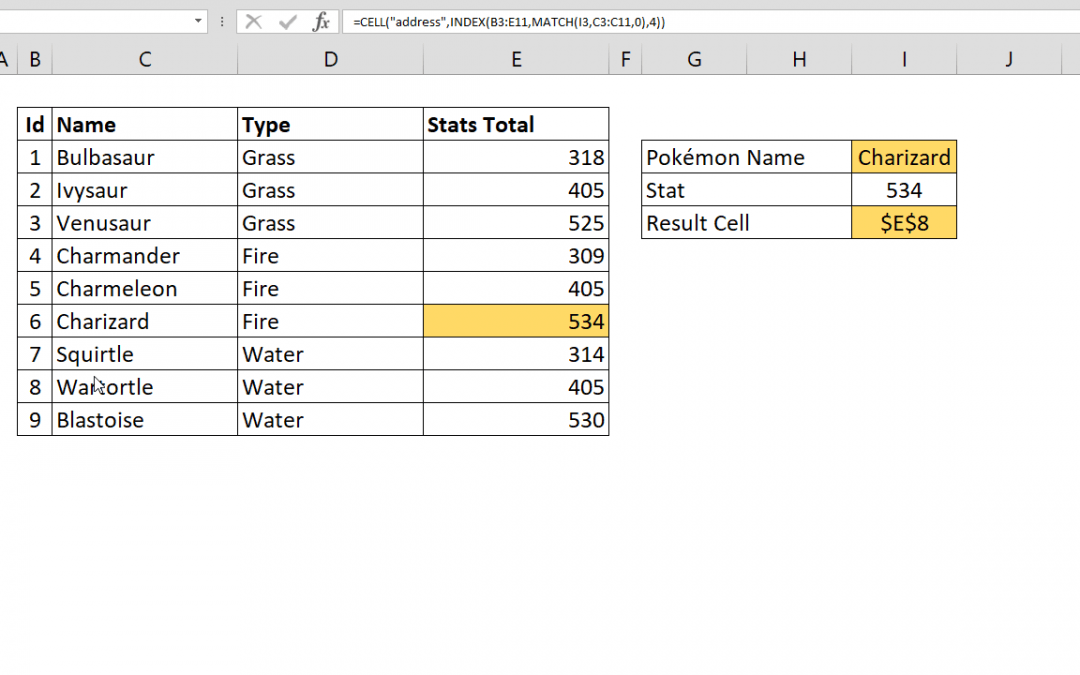
The CELL function can return various information about a cell reference. It uses 2 arguments. The first one specifies the type of information, the second one represents the cell reference. To get Excel cell address of a cell, we use "address" string as the first argument. We will use the INDEX function to get the second argument.

The INDEX function can return a value or the reference to a value within a range. Fortunately; you do not need to specify what the INDEX function will return. Excel automatically chooses between the value and the reference according which one is needed. All you need to do is to use your own lookup function inside a CELL function. For example;

=INDEX(B3:E11,MATCH(I3,C3:C11,0),4) returns 534 value

=CELL("address",INDEX(B3:E11,MATCH(I3,C3:C11,0),4)) returns $E$8 reference

For detailed information and example for the INDEX function, please see INDEX & MATCH: A Better Way to Look Up Data

This is a unique ability of the INDEX function. You cannot use the same trick on other lookup functions like the VLOOKUP or the MATCH.