Creating a dynamic Excel drop down list is very useful If you have a list that is updated frequently. This article shows you how to create a dynamic drop down list with the help of OFFSET and COUNTA functions.
Syntax
=OFFSET(title of list, 1, 0, COUNTA(column that includes the list)-1)
Steps
- Click Define Name under FORMULAS tab in ribbon
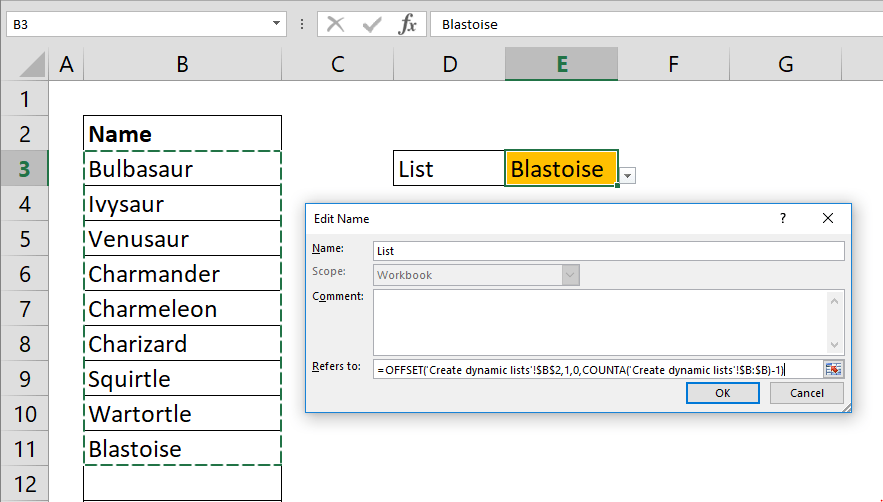
- Enter a name and clear Refer to formula box
- Start formula with the =OFFSET( function
- Select title of your list 'Create dynamic lists'!$B$2,
- Type 1, to make the list start at the next row, after the title
- Type 0, to make the list start in the same column
- Continue with COUNTA( function to count filled cells
- Select the whole column that includes the list 'Create dynamic lists'!$B:$B
- Type )-1 to close the COUNTA function
- Type ) to close the OFFSET function and finish the formula
- Click OK to save the name.
- Select the cell that will contains the drop down
- Click Data Validation under DATA tab in ribbon
- Select List in Allow drop down
- Type your name into Source box, with an equal sign =List
- Click OK to save data validation
How
We are using the OFFSET function's ability to return arrays to generate dynamic lists. Using COUNTA function to return row count gives the entire formula the dynamic behavior we are looking for
The OFFSET function returns an array that starts from a specified reference and has specified height and width numbers. The first argument of the OFFSET function is a base reference followed by Rows and Cols arguments which defines the array's top left reference. For example; If the first argument is C5 and the other two arguments are -1 and 2 respectively, it refers to cell E4 which is 1 row above, 2 columns right.
After determining where the array starts, next two arguments, which are 4th and 5th, defines the size of the array. If we continue with the same example;
=OFFSET(C5, -1, 2, 3, 4) formula refers E4:H6 range.
We can make this output range dynamic by making its size dynamic. Because we have a vertical list through column B, we should make 4th parameter, which refers to its Height, dynamic. The COUNTA function can help us to find the size of the list. Counting all nonblank cells in column B gives the size of our list. But, If your list contains a title which you may not want to include, decrease the value from COUNTA by 1 to eliminate the title.
Let's analyze our formula;
=OFFSET('Create dynamic lists'!$B$2,1,0,COUNTA('Create dynamic lists'!$B:$B)-1)
| Argument | Description | Return |
| $B$2, | Base reference is $B$2 | $B$2 |
| 1,0, | Return array starts from 1 row below (1) and at the same column (0) | $B$3 |
| COUNTA('Create dynamic lists'!$B:$B)-1 | Return array's size is the row number that returns from COUNTA('Create dynamic lists'!$B:$B)-1 | $B$3:$B$11 |
To create a dynamic drop down list in Excel, you need to use this formula in Data Validation. You can write the formula directly, however saving it in a name first makes it re-usability.
Also see the related article Excel’s Dynamic Charts: A Tutorial On How To Make Life Easier.