A common way to populate lists or tables in Excel is using the INDEX function. However, you need to create a helper column or row, to define row and column numbers for the INDEX function. This way, the INDEX can populate return the values into the corresponding cells. With Excel's new SEQUENCE function, this additional step is no longer necessary. In this article, we are going to show you how to create an Excel dynamic list or table, without the need of helper columns, and instead using the Excel auto generate number sequence dynamic array function: SEQUENCE.
Creating an Excel Dynamic List Using the SEQUENCE Function
To create an Excel dynamic list or table, we begin with the SEQUENCE function. The SEQUENCE function is one of the dynamic array functions Microsoft announced on September, 2018. A Dynamic Array function can populate an array of values in a range of cells, based on a formula. This behavior is called spilling, and can help overcome the limitations of traditional array formulas.

The SEQUENCE function can generate a list of sequential numbers in the form of an array or a range. It takes 4 arguments. Only one of them, row, is a required input, and the others are optional arguments that can be omitted.
Syntax
| rows | The number of rows to be returned. |
| [columns] | Optional. The number of columns to be returned. The default value is 1. |
| [start] | Optional. Starting value. The default value is 1. |
| [step] | Optional. The increment of each step between values. The default value is 1. |
Sample
You can generate a column of values using only the row argument. For example:
Use the column argument as well to generate an array that can fill columns. To generate a 1-row, multi-column array, use the following:
Populating an Excel Dynamic List or Table without Helper Columns
The INDEX function can get a value of from an array or a range in the specified coordinates. With this, it is possible to create a list or a table if you provide the coordinates for its row and column arguments. In the traditional method, you would need to create a helper column of sequential numbers and to use the reference of the column in an INDEX function. Basically this approach entails 4 steps:
- Create a helper column
- (Optional) Create a helper row if you want to populate a table
- Write the formula containing the helper column (and row) references
- Copy the formula along the helper column (and row)
The alternative approach we are mainly interested in today is using the SEQUENCE formula. When you type in this formula, Excel will spill the results automatically. Here is a sample formula to populate cells with the 5-row, 3-column version of a range named "SourceTable":

If you need to generate a list, use only the row argument. Here is a 4-row version of the column named "Type":

The examples we've covered here are only the tip of the iceberg when it comes to all kinds of things you can do with dynamic array functions. See our other tips and how-to articles for other examples.