The Excel FILTER function is a lookup and reference function that filters a range or array. The FILTER function is one of the newest Dynamic Array functions which are release with Excel 2019. In this guide, we’re going to show you how to use the Excel FILTER function and also go over some tips and error handling methods.
Supported versions
- At the time of writing this article, Microsoft announced that this formula is currently only available to a number of select insider users. When it's ready, the feature is planned for release for Office 365 users.
Syntax
Arguments
|
array |
The range or array you want to filter. |
|
include |
A Boolean array where TRUE values represent the return results. The include array should have the same height or width as the array argument. |
|
[if_empty] |
Optional. A return value for when the filter returns nothing. |
Examples
Note that we're using named ranges in our sample formulas to make them easier to read. This is not required.
Filter by row
Excel will populate the sorted list automatically. You do not need to select the range or specify how many items are to be listed. If there is enough space (empty cells) underneath the formula, the formula will work as intended.

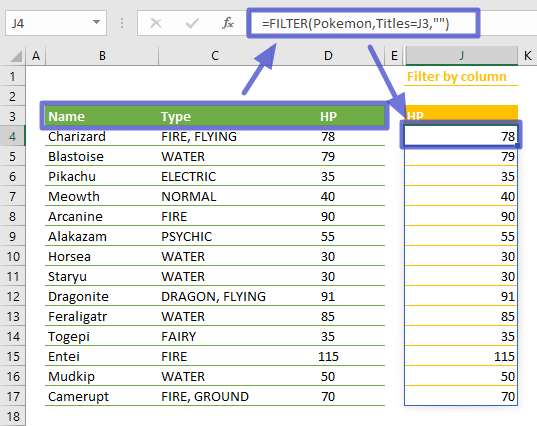
Filter by column
Filter by multiple columns

Dependent Dropdowns
=FILTER(Name,Type=DropdownType,"No Name Found")
- Use the UNIQUE function to generate a list for the first dropdown.
- Bind that list to a cell named DropdownType using Data Validation List.
- Use the FILTER function to filter the Name range by Type selected in the DropdownType.
- Bind the list of filtered values to a cell that is to be the dependent dropdown.
Whenever the DropdownType is changed, the list of the second dropdown will be updated.

Tips
- The Excel SORT formula can be used as an alternative to the Filter feature without modifying the actual data.
- Use * for logical AND, and + for logical OR for multiple conditions.
Issues
#SPILL!
If there isn't enough space for adding the results below the formula, you will see a #SPILL! error. Excel marks the target range with dashed lines. Clear the contents of the cells in this range, and Excel will automatically update the results.

#CALC!
If the filter returns no results and the [if_empty] argument is omitted you will get a #CALC! error.
#VALUE!
If the [include] value is not a Boolean value or array you will get a #VALUE! error.