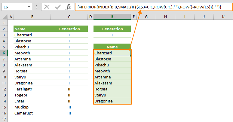
Filtering data helps focusing on certain aspects of a data set. Excel has built-in features for this, an Excel formula for filtering data was not in the software's scope until the introduction of dynamic array functions. In this guide, we’re going to show you how you can use Excel formula for filtering data.

Syntax
Steps
- Select the range of cells that will be populated with filtered values
- Start the formula with = IFERROR( function to return empty string when an error occurs)
- Continue with INDEX(
- Select or type in the range reference that contains your original list B:B,
- Continue with the SMALL( function which provides the row indexes of cells
- Next, use IF( to return an array that contains the numbers and empty strings
- Use an equation to filter $E$3=C:C, the criteria cell should be an absolute reference
- Continue with ,ROW(C:C),""), which will provide TRUE/FALSE conditions for the IF function
- Type in ROW()-ROW(E5) to generate an incremental number for array from the IF function
- Type in )),"") and press Ctrl + Shift + Enter to complete the array formula
How
To filter out values from a range, we need to pinpoint the cells that meet a certain condition, and retrieve them from the original list. Keep mind that we're going to need to create an array formula to avoid to creating several helper columns, and use a single Excel formula for filtering data. As a result, the formulas will return array values.
Our example returns values from column B by searching the value of cell E3 in column C. This condition leads to the logical test,
This test returns an array of Boolean values (TRUE and FALSE). For example, if the value of cell E3 is "I", the logical test returns an array like below,
{FALSE;FALSE;TRUE;TRUE;TRUE;…….;FALSE}
These Boolean values become the logical test values for the IF function. The IF function provides the row numbers of cells that meet the criteria, and returns empty strings for others.
The IF function here returns an array. This time an array of row numbers and empty strings.
{"";"";3;4;5;…….;""}
The next step is sorting the row numbers in our new array. The SMALL function can return the nth smallest number from an array. Also note that Excel evaluates string values as almost infinitely large numbers, making any other number small in comparison. This is the reason why the SMALL function is used instead of the LARGE function. To assign an 'n' value to the SMALL function, we use the ROW function again with a single cell that should be one cell above the first row to return numbers from 1, and use a relative reference to increase its row number. As a result; SMALL(IF($E$3=C:C,ROW(C:C),""),ROW()-ROW(E5)) formula returns a row index value which will be used by the INDEX function to return a value from a non-empty cell.
{1}
The INDEX function selects the reference to return values, and the IFERROR envelops the nested formula to avoid errors.
Finally, press the Ctrl + Shift + Enter combination instead of just pressing the Enter key to enter your formula as an array formula, and you're done!