The Excel LOOKUP is a Lookup & Reference formula that can search a value inside a column or row, and return a matching value from the same position in another column or row. In this guide, we’re going to show you how to use the Excel LOOKUP function and also go over some tips and error handling methods. The LOOKUP function has two forms: Vector form and Array form.
LOOKUP Function: Vector Form
The vector form is especially useful for searching a value inside a single row or column. A vector in this context means a single-dimensional row or column. In the vector form, you can specify the lookup and result vectors.

LOOKUP Function: Array Form
Microsoft strongly recommends not using the array form of the Excel LOOKUP function. Instead, it is recommended to use VLOOKUP or HLOOKUP functions, or the INDEX-MATCH combination. Excel retains the array form for compatibility reasons.
The array form allows using a table, instead of a vector. The array form searches the specified value in the first column or row of the array, and returns a value from the same position in the last column or row of the array.

Supported versions
- All Excel versions
Excel LOOKUP Function Syntax
lookup_value: This is the value you're searching for.
lookup_vector / lookup_array:
Vector form: This vector includes the lookup value.
Array form: This array encompasses both the lookup and result values.
[result_vector]: (Optional) This is the vector containing the return value.
Examples of LOOKUP Function
The examples below use the vector form of the LOOKUP function. You can also find array form examples in our sample workbook linked below.
Row Search with LOOKUP Function
To use the vector form of the Excel LOOKUP function, you need to provide the value you want to search and two vectors (two one-dimensional vertical ranges). The first vector specifies the where the lookup_value will be searched, and the other one includes the return values.
In our example, we want to get the Stats value of a specific Pokémon by searching for its name. In this scenario, our formula would be like below.
The function searches for the value "Charizard" in a row vector, named Name, and returns a value from the same position, in a row vector Stats. The result is 534.

Column Search with LOOKUP Function
To perform a search inside a column, the LOOKUP function's vectors should be one-dimensional horizontal ranges. For example, the formula below searches for the string "Type" in a vector named TitleRow, B2:D2. If the function finds the value, it returns the corresponding value in a vector named CharizardRow, B7:D7. The golden rule here is using vectors of equal size.

Error Handling in LOOKUP Function
Here are some common error scenarios related to the LOOKUP formula and how to handle them:
#N/A Error: This is the most common error with the LOOKUP function. It occurs when the function fails to find the lookup_value in the lookup_vector. This can happen if the value doesn't exist in the vector or if the vector isn't sorted correctly (for approximate matching). To handle this error, you can use the IFNA function to provide an alternative result when an #N/A error occurs. When using the vector form of the LOOKUP function, the lookup_vector and result_vector must be of the same size. If they aren't, Excel returns an #N/A error. Always ensure that both vectors are of equal length.
#REF! Error: This error occurs if the result_vector range is invalid (for example, if it references a deleted cell). Check the integrity of your data ranges to avoid this error.
Data Sorting Issues: The LOOKUP function assumes that the lookup_vector is sorted in ascending order for an approximate match. If the data isn't sorted, the function may return incorrect results or an #N/A error. Ensure that your data is sorted correctly, or use an exact match function like VLOOKUP or INDEX-MATCH with FALSE or 0 as the last argument for exact matching.
Type Mismatch: Sometimes, the type of the lookup_value might not match the types of values in the lookup_vector (for example, looking up a text value in a range of numbers). Ensure that the data types are consistent to avoid errors.
Tips
- Refrain from using the array form, and use VLOOKUP, HLOOKUP or INDEX-MATCH instead.
- The LOOKUP function does an approximate search. This means,
- The function assumes the lookup_vector is sorted in ascending order.
- It returns the next smallest value when lookup_value is not found.
- When lookup_value is greater than all values in the lookup_vector, the LOOKUP matches the last value.
- Regardless of the orientation, the result_vector must be the same size as the lookup_vector.
- The lookup_vector can be a horizontal range when the result_vector is vertical, and vice versa.
- Excel LOOKUP function is not case-sensitive like other lookup formulas.
Other Lookup Functions
In Excel, there are several alternative formulas to the LOOKUP function, each with its unique features and use cases. These alternatives can be more suitable depending on the specific requirements of your data analysis or the complexity of your dataset.
VLOOKUP Function - Vertical Lookup
The VLOOKUP (Vertical Lookup) function in Excel is designed for vertical data searches within a specific column. It locates a value in the first column of a table and returns a corresponding value from another column in the same row. The syntax is
=VLOOKUP(lookup_value, table_array, col_index_num, [range_lookup])
where lookup_value is the value to search for, table_array is the range containing the value, col_index_num is the column number from which to retrieve the value, and [range_lookup] is an optional parameter to specify exact match (FALSE) or approximate match (TRUE). VLOOKUP is user-friendly but has limitations, such as only searching in the first column and moving rightward, and it can't handle column insertions or deletions gracefully.
HLOOKUP Function - Horizontal Lookup
HLOOKUP (Horizontal Lookup) works similarly to VLOOKUP but is tailored for horizontal data searches. It finds a value in the first row of a table and returns a value from the same column in a specified row. The syntax
=HLOOKUP(lookup_value, table_array, row_index_num, [range_lookup])
includes lookup_value (the value to find), table_array (the data array), row_index_num (the row number to retrieve the value from), and [range_lookup] for exact or approximate match. HLOOKUP is beneficial for horizontally structured data but has similar limitations to VLOOKUP in terms of flexibility and adaptability to data structure changes.
INDEX and MATCH Functions
The INDEX and MATCH combination offers more flexibility than VLOOKUP and HLOOKUP functions. MATCH locates the position of a lookup value in a column or row, and INDEX returns a value from a specific position in a range. The typical syntax is
=INDEX(range, MATCH(lookup_value, lookup_range, [match_type])).
This combo overcomes the limitations of VLOOKUP and HLOOKUP, as it can search in any column or row and is not disrupted by column or row insertions. It’s particularly useful for complex data sets where you need to search across multiple columns or rows.
XLOOKUP Function
XLOOKUP, available in newer Excel versions, is a highly versatile function that simplifies and enhances lookup capabilities. It performs both vertical and horizontal lookups and replaces the need for VLOOKUP, HLOOKUP, and INDEX/MATCH. Its syntax,
=XLOOKUP(lookup_value, lookup_array, return_array, [if_not_found], [match_mode], [search_mode])
provides straightforward parameters for the lookup and return arrays, and optional arguments for unmatched values, match types, and search modes. XLOOKUP's ability to search in any direction and handle array returns makes it a powerful tool for modern Excel users.
FILTER Function
Exclusive to Excel 365 and Excel Online, the FILTER function is designed for extracting specific data based on given criteria. It filters a range based on the criteria and returns an array of matching values. The syntax is
=FILTER(array, include, [if_empty])
where array is the range to filter, include specifies the criteria, and [if_empty] provides a value if no matches are found. The FILTER function is particularly powerful for dynamic arrays and when dealing with complex criteria, as it can return multiple results that meet the specified conditions.
CHOOSE Function
The CHOOSE function is a straightforward method for selecting one of several values based on an index number. Its syntax,
=CHOOSE(index_num, value1, [value2], ...)
allows users to specify an index number and a list of values, where index_num decides which value is returned. CHOOSE is simple and effective for scenarios where you need to switch between a set of predefined options based on an index. It's less about searching data and more about selecting from a list of alternatives.