Excel MOD Function

The Excel MOD function is a Math and Trigonometry formula which calculates and returns the remainder after the number is divided by the divisor. This is called a modulo operation. This operation sees frequent use in math problems and building a model, and you can use the function to do things like making calculations on the nth values in a list. In this guide, we’re going to show you how to use the MOD function and also go over some tips and error handling methods.

Supported versions

• All Excel versions

Excel MOD Function Syntax

Arguments

Function Examples

Basic Use Case

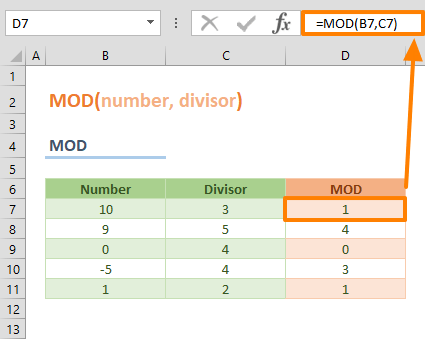
The function requires two arguments: number and divisor. Excel divides the number argument by the divisor value, and returns the remainder in the cell. For example, to calculate the remainder value for dividing 10 by 3, the following formula can be used:

Alternative Use Cases

An alternative use case for this function is for running calculations using the nth-values from a data list. For example, you can use this function to sum the cell values with only even row numbers.

Let's say we have a list of numbers in the range B7:B11. The even row numbers in this range are 8 and 10. Using this function in conjunction with the ROW function, you can return the row number. The row number would be an even number, if MOD returns 0, when the divisor parameter is set to 2.

By default, neither the MOD, nor the ROW functions allow using arrays. You need to use them with an array formula or inside another function that can evaluate arrays. One function you can use here is SUMPRODUCT. The SUMPRODUCT function multiplies the values in arrays, and returns the sum of products. However, we only need it for its array handling abilities in this example.

The following function sums every cell value with even row numbers in a named range called list:

(MOD(ROW(list),2)=0) part generates an array of TRUE and FALSE values. Multiplying logical values with the array itself returns sum of the numbers corresponding with TRUE values.

In a similar manner, if you want to calculate the nth-value­ in a list, you can use the same formula with some modifications:

1. Replace the divisor value with the n-value­. For example, use 3 to calculate every 3^rd value.
2. Subtract the first row number from the range to eliminate the actual row numbers. For example, if the range starts from the 7^th row, use ROW(list)-7.

With these changes, the formula becomes:

Download Workbook

Tips

• The function always returns a result with the same sign as the divisor.
• The function is often seen in formulas that deal with every nth-value.

Issues

• The MOD function will return a #DIV/0! error if the divisor is zero (0).