Users of all levels have different feelings about Excel named ranges. Some find them cumbersome, while others use them religiously.

In addition to allowing quick access to complex references, named ranges can make your formulas a lot easier to read and maintain. Once you make the habit of using named ranges in your Excel workbooks, you’re going to feel the difference in how quickly you can work and manage your data.

In this article, we’re going to cover the basics, advanced features, and various ways of how Excel named ranges can make life easier. We’re going to be using different examples for each feature. Please feel free to download our sample workbook below.

What is a Named range?

Named ranges are cells, ranges, tables, formulas, or constant values that are represented with meaningful names, besides their workbook reference (i.e. A1, B23, A1:B23). Using named ranges make formulas easier to read and maintain.

Let's take an example. Here we have a formula using INDEX function that looks up a value.

=INDEX(B3:E11,MATCH(I3,C3:C11,0),4)

Using named ranges, this formula would look like below.

=INDEX(sales_data,MATCH(current_date,dates,0),amount_column)

The second example is easier to interpret as you don’t need to go back to that specific reference and identify what these cell references are.

Creating Named Ranges

There are several ways to create Excel named ranges. The easiest method is selecting the cell range, and then typing in the name of your named range into the reference box (right before the formula box on the top bar).

Please note that there are certain limitations for what names you can use as a named range. Consider the items below when creating named ranges.

The first character of a name must be a letter, an underscore character ( _ ), or a backslash ( \ ).
The subsequent characters in the name can be letters, numbers, periods, and underscore characters.

Note: Although you can create names that consist of a single letter, such as "a", "e" or "j"; you cannot use the uppercase and lowercase characters separately (i.e. "C", "c", "R", or "r").

Names cannot be the same as a cell reference (i.e. Z$100 or R1C1).
You can’t use a space.
A name can contain up to 255 characters.
Names are NOT case sensitive. According to Excel "data", "Data" and "DATA" are the same.

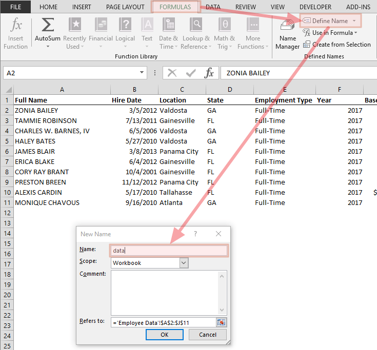
Another way to create a named range is by going into the Define Name menu from the FORMULAS tab in the ribbon. First select your cell, then go to this menu and type in the desired name into Name box and click OK to apply.

Note: The same New Name dialog will pop up if you click the New… button in the Name Manager window. Follow these steps to create a name using the Name Manager:

Go to the FORMULAS tab in the ribbon
Click Name Manager
In the Name Manager window, click the New… button

If you want to add several named ranges in one go, go to Create Names from Selection. This feature allows you to add name ranges using the labels adjacent to your ranges. To do this:

Select your data
Go to the FORMULAS tab in the ribbon
Click Create Names from Selection
Select options that applies to your data. For example, selecting Top row and Left column options will give 5 named ranges in our example:
1. Inputs =B2:B5
2. First_Name =B2
3. Last_Name =B3
4. Age =B4
5. Occupation =B5
Click OK to add named ranges

Note: If the labels next to selected cells do not meet the limitations mentioned before, Excel automatically removes unsupported characters and replaces them with underscore characters ( _ ). As a result, "First Name" in this example was registered as "First_Name".

Use Cases

References

Named ranges are typically used for giving meaningful names to cell and ranges. You can use those names like regular references without having to use the actual cell range references.

sales_data = B3:E11

current_date = I3

dates = C3:C11

Constants

Just like cell and range references, constant values can also be used as named ranges. Instead of entering a commonly used value every time, entering a name instead can be easier and make your formulas easier to understand.

To save a constant value as a named range you need to use the Name Manager. In Name Manager window, click the New… button, and type in the value after an equal sign into the Refers to: panel.

Formulas

Formulas can also be given named ranges. You can create a named range from a formula the same way you would with constant values using the Name Manager.

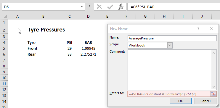
Entering your formula after an equal sign in the Refers to section will save this entire formula as a name.

This ability shines especially when creating dynamic ranges that can grow or shrink automatically based on workbook data. For example, =OFFSET(Sheet1!$A$1,0,0,COUNTA(Sheet1!$A:$A),1) formula in this example returns an array of values and excludes spaces, when you enter data into column A. With this formula, you can create dynamic dropdown lists or dynamic charts without unnecessary spaces. Using a named range instead is certainly faster than using the entire formula. For more information about dynamic charts check out our Excel’s Dynamic Charts: A Tutorial On How To Make Life Easier article.

Tables

When you add a Table, more accurately, when you convert your data into a Table, Excel automatically adds a Named Range that refers to that table. Although table names are listed in Name Manager, they differ from regular Excel Named Ranges – You can't edit the reference range or delete it from the Name Manager window. Table named ranges are also shown with a different icon than named ranges.

Table named ranges are dynamic by default, so they can grow and shrink as you add or remove data. To add a table and use this functionality, just select your data and press Ctrl + T and follow the steps.

Other Advantages

Names in formulas list

Named Ranges are automatically listed in the formulas list when you start typing.

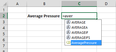
Even if you have long named ranges, you can select them quickly for using them in formulas. Pressing the Tab key will add it to your formula automatically.

Call a name from name list

There is an alternative to using named ranges in formulas method which allows you to see only named ranges in a separate list and add them to your formula. While typing in a formula, press the F3 key to bring up the Paste Name list.

Select the named range and click OK to add it.

Copy formulas between workbooks and worksheets

Excel named ranges make working between several workbooks and worksheets a breeze. For example, if you have similar workbooks that cover user input data from different years, you might want to use similar formulas with different range references. When applying the formulas from one worksheet to another, you need to update the formula ranges manually. However, if you use names instead of references and use the same names for similar data, the copying process will be much easier as formula syntax will remain the same between workbooks.

The same approach can be used between worksheets as well. However, in this case, named range scopes should be selected as “worksheets”, instead of “workbook”. We will cover named range scopes later in this article.

Navigation

Named Ranges are useful for fast navigation. All named ranges are listed in the dropdown menu under the reference box. Clicking a name will automatically move your focus to the named range.

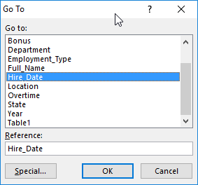
Named ranges are also listed in the Go To window. Press F5 to open the Go To window and double click the name you want to go to.

Named can be used as hyperlinks

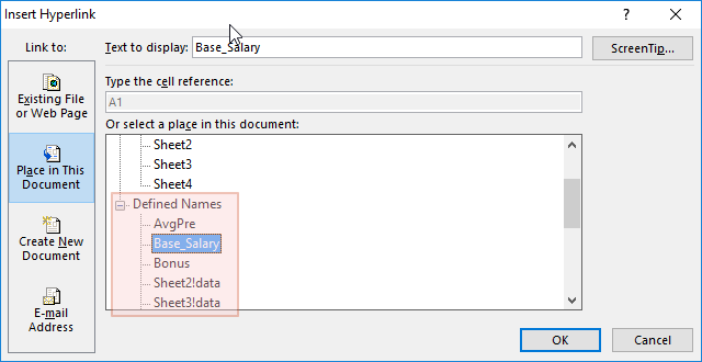
Named Ranges will appear in the Insert Hyperlink window. To add a hyperlink;

Right-click the cell
Click Hyperlink from the menu
In the Hyperlink window, click Place in This Document
Select the name you want to link and click OK

An alternative way to create hyperlinks is to use the HYPERLINK function. You can use Named Ranges in HYPERLINK function by placing a hash character (#) before the name.

=HYPERLINK("#State","Go to State List")

Dynamic Ranges via tables

We’ve already learned that dynamic ranges can be created using formulas and a Named Range. An alternative way to do this is by using a Table reference inside a Named Range. We’ve mentioned that table named ranges are dynamic and can automatically grow or shrink, and we will be using this feature to do the same for a single named range.

Tables have their own reference syntax. Table name comes first and column name follows, inside brackets. For example, "Table1[State]" refers to column name "State" in "Table1". Because this table is dynamic, its columns will be dynamic as well. The trick is creating a Named Range that refers to a table reference, instead of a single range reference or a formula.

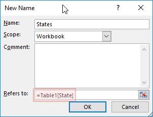
"States" named range is now a dynamic range too.

Zoom out to see Excel Named Ranges

If you have data that spans over dozens of rows and/or columns, giving those tables named ranges and zooming out can help visualize the big picture. Excel starts showing names when the zoom level is below 40%.

Scope

Named Ranges can be defined under workbooks or worksheets. This is the scope of the named range. Scope of named ranges are Workbook by default.

‘Workbook’ scope means you can access the specified named range from all sheets and it always refers to the same value, formula, or reference.

On the other hand, if a named range's scope is set to ‘worksheet’, that name works inside that specific worksheet. This feature is useful when you have same kind of data across different worksheets. Excel allows giving the same name into multiple ranges as long as they are not under overlapping scopes. The example below contains 3 named ranges, all of which are named "data".

=SUM(data) formula returns 3 different values when the formula is used in each sheet (i.e. Sheet2, Sheet3, Sheet4).

In Sheet2, =SUM(data) returns 10
In Sheet3, =SUM(data) returns 110
In Sheet4, =SUM(data) returns 1110

To call a local scoped named range from different worksheet, you need to use the parent worksheet name as well. For example:

In Sheet2, =SUM(Sheet2!data) returns 10
In Sheet3, =SUM(Sheet2!data) returns 10
In Sheet4, =SUM(Sheet2!data) returns 10

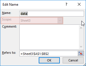
You can determine the scope of a named range when you add it. You need to use Define Name menu or the Name Manager to add a local scoped named range. In the New Name menu, choose a worksheet under the Scope dropdown.

Please note that you can’t change this afterwards. The only way to do this by deleting the named range and create it again.

How to manage and delete Excel Named Ranges

The Name Manager window is like the base of operations for Named Ranges. Here, you can find a list of all named ranges, add/edit/delete them.

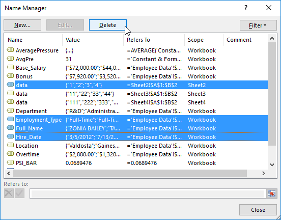
Deleting Named Ranges

To delete name ranges, first select names you want to delete, and then click the Delete button. You can use Ctrl and Shift keys to select multiple names and delete them with one click.

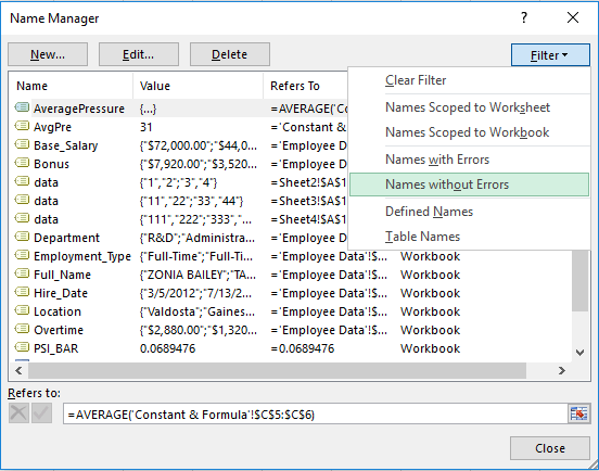
Filtering and sorting names

Name Manager allows sorting and filtering names. You can sort names by clicking the columns for Name, Value, Refers To, Scope or Comment.

Multiple filters can be applied from the Filter dropdown.

Additional Features

Apply Names

If you create named ranges after creating your formulas, the formulas will keep using regular references if you do not update them. To update formulas, you have 2 options:

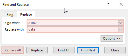
Changing references using the Find & Replace
Using Apply Names feature

For the first method, open the Find & Replace dialog (i.e. Ctrl + F), then enter reference and named range. Click the Replace All button to replace all occurrences.

The second method is a bit easier and, in some cases, safer than Find & Replace because you don't need to enter a reference. To use Apply Names, click the down arrow next to the Define Name under FORMULAS tab and go to Apply Names. This will bring up the Apply Names window with a list of names. Select the names you want to update and click OK to convert ranges into names automatically.

Paste List

You can open the Paste Name dialog by pressing the F3 key on your keyboard, or find it under the Use in Formula dropdown in the FORMULAS ribbon.