SUMIFS like other …IF or …IFS function are great tools to aggregate data based on a set of conditions. The downside of this approach is that the criteria must be supplied manually, especially when you need to create a summary table. In this guide, we’re going to show you how to use UNIQUE and SUMIFS functions in combination to generate an Excel summary table.
A summary table should include a unique list of categories. Creating a unique list of categories can become tedious as you keep adding more items in the future. To keep things simple and automate this task, you essentially can use either one of the two methods: Pivot Table or Excel formulas. Let's take a look at both.
Formula approach
Although Excel has a built-in feature for creating unique lists (or rather removing duplicate values), this actually requires a more manual approach. There were no dedicated formulas or tools since 2018 for creating a unique list of values. Traditionally, you had to use complex formulas to get a list of unique items.
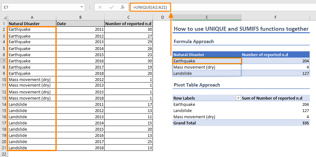
Fortunately, Microsoft has introduced the UNIQUE formula in the later versions, which makes things much easier and automates most of this process. All you need is to do is to supply the reference of categories in your data. Excel will populate the unique list of values automatically.
=UNIQUE(A2:A21)
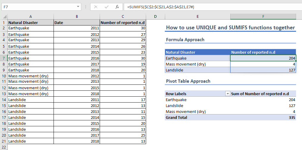
Once the unique list is ready, you can use SUMIFS function which will use the generate the unique list. The trick is to use the spill operator for the criteria argument (E7#). With the spill operator, SUMIFS function will gain a dynamic array and start to populate automatically with unique list of items. You won’t need to copy the SUMIFS formula down to the list.
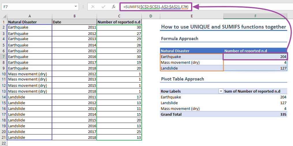
Pivot Table Approach
An alternative way to creating an Excel summary table is using a PivotTable. A PivotTable automatically creates a unique list of category items and aggregates the data. The approach is simple:
- Select any cell in your data set
- Click Insert > PivotTable
- Select the cell / worksheet where you want to place the PivotTable
- After the PivotTable field is created, use the right panel (Field List) to add fields into the table area. In our example, we moved categories to the Rows section and values to the Values section
- Update the aggregation method based on your needs. The default method is to sum for numeric values.