Excel Table is a tool for managing and analyzing data in tabular format. An Excel Table provides the data in a special structure, which includes filtering, formatting, sizing, and auto populating formulas dynamically. In this guide, we're going to go over some tips and tricks you can use with Excel Tables for better results and efficiency.
1. Easy to create
Creating a table, or more converting a regular range of cells into a table is an easy process.
- Select a cell inside your data range
- Press Ctrl + T
- Make sure My table has headers checkbox is checked if your table has headers
- Click OK to convert your range into a table
Alternatively, you can use the Table icon from the INSERT tab of the Ribbon.

2. Auto-expansion
An Excel Table automatically expands when you enter new rows or columns. This way you can have dynamic ranges or lists that can be used in formulas and data validation lists.

3. Auto-fill/update formulas
A formula entered inside a column is applied to all cells in that column automatically. You do not need to copy & paste or use autofill.

4. Structured references
Excel uses a special formula syntax rather than A1-style to refer to tables. This feature is called "structured references". Structured references looks like named ranges that are automatically created with the table.
Thanks to structured references, you do not need to remember the exact cell references when using them in formulas. For example, to use the HP column from our example as an argument for the SUM function, we can click on a title of the column. Excel will typically list possible name tags as you type.

5. Rename a table
Excel gives the table a generic name when it's first created (i.e. Table3). Changing the table name can be useful to help you remember when you referring a table via structured reference. The table name will be updated in all existing formulas.

6. Total Row
You can add your tables a row for totals without actually using any formulas. This feature is called Total Row and follows the same idea as using the SUBTOTAL function by default. You can choose the calculation type from a dropdown or add your own formula. The Total Row always remains at the bottom of the table even when the table expands or shrinks. So, you do not need to update the formulas every time. To add this row, activate the Total Row by clicking the Total Row checkbox in the DESIGN tab for the table.

7. Navigation to a table
Excel treats tables similar to named ranges. You can use this property to find a table just like finding a name. The name of a table can be found in the reference / name box next to the formula box, as well as from the Go To window which can be accessed by pressing the F5 key. You can find a table's name in the Paste Name (shortcut: F3) dialog.

8. Shortcuts in tables
Shortcuts can be used when a cell or range in the table is selected. For example, the Ctrl + + combination pops up the Insert dialog with options. However, when used in a table, Excel directly adds a new row into the table. Below is a list for the shortcuts.
|
Action |
PC |
Mac |
|
Insert table |
Ctrl T |
⌃ T |
|
Toggle Autofilter |
Ctrl Shift L |
⌘ ⇧ F |
|
Activate filter |
Alt ↓ |
⌥ ↓ |
|
Select table |
Ctrl A |
⌘ A |
|
Select table row |
Shift Space |
⇧ Space |
|
Select table column |
Ctrl Space |
⌃ Space |
|
Insert rows |
Ctrl Shift + |
⌃ I |
|
Insert columns |
Ctrl Shift + |
⌃ I |
|
Delete rows |
Ctrl - |
⌃ - |
|
Delete columns |
Ctrl - |
⌃ - |
9. Moving a row or column by dragging and dropping
You can rearrange rows and columns by dragging & dropping . Just select the row or column you want to move, and drag it to the desired place. Make sure that the header is also selected before moving a column.

10. Table headers
The headers can be replaced with column identifiers when you scroll down the page.

11. Formatting
When a table is selected, Excel will show a new tab named Design under the Ribbon. You can find preset formatting options under the Table Styles section. Feel free to customize them as you need.

12. Slicer
Slicers are commonly used in Pivot Tables, and they can be used in tables as well. A slicer essentially filters data by item group. You can easily add a slicer by using the Insert Slicer icon in the Design column when the table is selected.

13. Remove a table (Convert to Range)
To remove a table or "convert the table to a range", right-click on the table and click on Convert to Range under the Table item. Alternatively, you can find the same command the Design tab of the Ribbon. If you don't want to keep the format of the table, select None for the table style and then Convert to Range.