Managing and organizing data in Excel doesn't have to be a daunting daily routine, especially when it involves tasks like finding unique values in your datasets. Unique values in Excel are those distinct, non-repeating entries essential for various data analysis tasks. They are the cornerstone in scenarios such as sorting through customer data, analyzing survey results, or managing inventory systems.
Identifying unique values in Excel is a vital skill for ensuring data integrity and eliminating redundancies. It's not just about mastering a specific function; it's about embracing a more efficient way to handle and understand your data. This capability in Excel can transform your approach to data analysis, making it simpler and more accurate.
In this article, we will guide you through finding unique values in Excel. This guide provides comprehensive insights into using unique values in data management. We aim to equip you with the knowledge and tools to streamline your data-handling tasks, helping you make more informed decisions based on clear, concise, and accurate data analysis.
Syntax
{ =IFERROR(
INDEX( data,
MATCH( 0,
IF( criteria=criteria list,
COUNTIF( mixed reference of on cell above,
data )),0)),"") }
The syntax you've provided appears to be a formula used in Excel to extract unique values based on certain criteria. It's an advanced formula that combines several functions: IFERROR, INDEX, MATCH, IF, and COUNTIF. Let's break it down for better understanding:
IFERROR Function: This function is used to catch and handle any errors in the formula. It takes two arguments - the formula you want to execute and the value to return if an error is encountered. In this case, the entire formula is the first argument, and an empty string ("") is the second argument. If any part of the inner formula fails, it will result in an empty string instead of an error message.
INDEX Function: The INDEX function returns a value or the reference to a value from within a table or range. Here, INDEX(data,...) returns a value from the 'data' range based on a row number that will be identified by the MATCH function.
MATCH Function: The MATCH function searches for a specified item in a range of cells and then returns the relative position of that item. In this formula, MATCH(0,...,0) looks for the first occurrence of the number 0 in an array provided by the IF function, indicating the first unique value.
IF Function with Criteria: This part of the formula IF(criteria=criteria list,...) is used to apply a certain condition. If the condition is met (i.e., the data in 'criteria' matches the 'criteria list'), it processes the next part of the function; otherwise, it ignores it.
COUNTIF Function with a Mixed Reference: COUNTIF(mixed reference of one cell above data) counts the number of times a specific value appears in a range. The mixed reference (like $A1:A1) increases the range as the formula is copied down a column. This part of the formula is crucial in identifying unique values.
Combining All Together: The formula is an array formula (denoted by curly braces {}), which processes multiple values simultaneously. It checks each cell in the 'data' range against the 'criteria' and 'criteria list.' Each cell that meets the criteria uses COUNTIF to see if it's the first occurrence. If it is, MATCH finds its position, and INDEX returns the value. If it's not a first occurrence or doesn't meet the criteria, the formula moves to the next cell. The IFERROR ensures that if there's an error (like no more unique values), it returns an empty string.
This formula extracts a list of unique values from a specified range ('data') that meet certain conditions ('criteria'). It's a powerful way to sift through large datasets and extract only the relevant, unique entries based on specific conditions.
Steps to Find Unique Values
Start with the IFERROR function: `=IFERROR(`. The `IFERROR` function is used at the beginning of the formula to handle any possible errors. It ensures that if any part of the formula results in an error, instead of displaying an error message, Excel will show an alternative result, which, in this case, will be an empty string.
INDEX function: `INDEX(`. The `INDEX` function returns a value from a specific place in a given range. This formula will return a value from the data list based on a position number that will be provided by the `MATCH` function.
Enter the data list reference: `$C$3:$C$11,`. Here you specify the range of your data list from which you want to extract unique values. This range is the area that the `INDEX` function will search to return the required value.
MATCH function: `MATCH(`. The `MATCH` function is used to find the position of a specified item in a range. This formula is used to find the position of the first unique value in the data list.
Type in 0 to get the unlisted value: `0,`. Typing in 0 here is crucial as it tells the `MATCH` function to find the first value in the range that has not been listed yet – essentially, the first unique value.
IF function maintains the condition: `IF(`. The `IF` function checks whether a certain condition is met. In this case, it's used to compare each value in the data list with a criterion.
Enter criteria-criteria list equation: `$F$2=$B$3:$B$11,`. This part sets the condition for the `IF` function. It compares each value in the range `$B$3:$B$11` with the value in `$F$2`. If a match is found, the function proceeds to the next step.
Continue with COUNTIF: `COUNTIF(`. The `COUNTIF` function counts the number of times a specific value appears in a range.
Enter the mixed reference for a range: `$H$2:$H4,`. This range reference contains the cell above and is used by `COUNTIF` to check if the current value has appeared before in the list of unique values.
Enter the data list reference again: `$C$3:$C$11`. Here, you re-enter the data list reference, specifying the range that `COUNTIF` should check for duplicates.
Close COUNTIF and IF functions: `)),.` This closes both the `COUNTIF` and `IF` functions.
Type in 0 for an exact match: `0`. This is used in the `MATCH` function to specify that you want an exact match.
Close both MATCH and INDEX functions: `)),`. This closes the `MATCH` and `INDEX` functions.
Add an empty string for error handling: `".` This is the value that `IFERROR` will return if there's an error in the formula, effectively preventing error messages from being displayed.
Close the IFERROR function: `)`. This closes the `IFERROR` function.
Finalizing as an Array Formula: Once you've entered the formula, press `CTRL + SHIFT + ENTER` on your keyboard. This combination is essential for creating an array formula in Excel, which processes multiple values simultaneously.
Copy the Formula Down: Copy it down the column after creating the array formula. This allows the formula to evaluate each row of your dataset, finding and listing unique values based on the specified criteria.
This expanded explanation provides a step-by-step guide on how the formula works, ensuring that each function and its purpose are clearly understood. By following these steps, you can effectively use this formula to extract unique values from your dataset in Excel.
How to Find Unique Values in Excel?
Let's break down and expand the explanation for the formula in cell H4:
`=IFERROR(INDEX($C$3:$C$11,MATCH(0,IF($F$2=$B$3:$B$11,COUNTIF($H$2:$H3,$C$3:$C$11)),0)),"")`.
This is an array formula used in Excel to extract unique values from a list based on specific criteria. It's designed to return a unique value from the range `$C$3:$C$11` that matches a criterion specified in `$F$2` and hasn't been listed in the previous cells (`$H$2:$H2`). Here's an expanded breakdown:
IFERROR(...,""): This function is wrapping the entire formula to handle any errors. If any part of the inner formula returns an error, `IFERROR` will result in an empty string ("") instead of displaying the error message.
INDEX($C$3:$C$11, ...): The `INDEX` function returns a value from the `$C$3:$C$11` range. The row number provided by the nested `MATCH` function determines the specific value returned.
MATCH(0, ..., 0): The `MATCH` function searches for the first instance of `0` in the array generated by the `IF` function. The zero signifies the first occurrence of a unique value that meets the criteria and hasn't been listed before.
IF($F$2=$B$3:$B$11, ...): This `IF` function checks if each value in the `$B$3:$B$11` range matches the criterion in `$F$2`. If a match is found, the `COUNTIF` function is executed; otherwise, it returns `FALSE.`
COUNTIF($H$2:$H3, $C$3:$C$11): This function counts how many times each value in the `$C$3:$C$11` range has appeared in the range `$H$2:$H3`. The `$H$2:$H3` range expands as the formula is copied down, ensuring that each cell checks all previous cells for the occurrence of the value.
Array Output {FALSE;1;FALSE;FALSE;FALSE;0;FALSE;0;FALSE}: The `IF` function combined with `COUNTIF` generates an array like `{FALSE;1;FALSE;FALSE;FALSE;0;FALSE;0;FALSE}`. Here, `FALSE` indicates values that don't meet the criterion set in `$F$2`, `1` (or any number greater than 0) indicates values that have already been listed before, and `0` indicates a unique value that matches the criterion and hasn't been listed yet.
How the Formula Works in Cell H4:
- The formula checks each value in `$C$3:$C$11` against the criterion in `$F$2`.
- It then uses `COUNTIF` to determine if each value has already appeared in the range `$H$2:$H3`.
- The `MATCH` function looks for the first `0` in the array, indicating a unique value that meets the criterion and hasn't been listed before.
- The `INDEX` function then returns this unique value.
- If no such value is found (all values are `FALSE` or greater than `0`), `IFERROR` results in an empty string.
Finalizing as an Array Formula: This formula must be entered as an array formula by pressing `CTRL + SHIFT + ENTER` on your keyboard, allowing it to process multiple values simultaneously.
Copying the Formula Down: By copying the formula down the column in your Excel worksheet, you can continue to extract the next unique values that meet the specified criteria.
This formula is particularly useful in scenarios where you need to extract a list of unique values from a larger dataset based on specific conditions, ensuring efficient data analysis and management in Excel.
| Steps | Formula Part | Description | Return Value |
| 1 | COUNTIF($H$2:$H3,$C$3:$C$11) | The COUNTIF returns an array that includes 1 for each existed value of $C$3:$C$11 in expanding $H$2:$H3 and 0 for not existed | {0;1;0;1;0;0;1;0;1} |
| 2 | $F$2=$B$3:$B$11 | The IF function's logical test argument generates another array that represents our criteria: $F$2=$B$3:$B$11 | {FALSE;TRUE;FALSE;FALSE;FALSE;TRUE;FALSE;TRUE;FALSE} |
| 3 | IF($F$2=$B$3:$B$11,COUNTIF($H$2:$H3,$C$3:$C$11)) | The IF function returns the values of array in step 1 according to its logical test results. If there is a TRUE value at same positon of array, value is listed. | {FALSE;1;FALSE;FALSE;FALSE;0;FALSE;0;FALSE} |
| 4 | MATCH(0,IF($F$2=$B$3:$B$11,COUNTIF($H$2:$H3,$C$3:$C$11)),0) | The MATCH function searches 0 in array and returns the exact position of matched value | 6 |
| 5 |
INDEX($C$3:$C$11, MATCH(0,IF($F$2=$B$3:$B$11,COUNTIF($H$2:$H3,$C$3:$C$11)),0)) |
The INDEX function returns the value in data range by using MATCH function's return value |
"John"
|
| 6 |
=IFERROR(INDEX($C$3:$C$11, MATCH(0,IF($F$2=$B$3:$B$11,COUNTIF($H$2:$H3,$C$3:$C$11)),0)),"") |
The IFERROR returns the INDEX function's result unless there is an error. |
"John"
|
Tips
When dealing with complex Excel formulas, like the one we've discussed for extracting unique values, how you enter the formula into Excel is crucial. Array formulas, an example of this particular formula, are designed to work with multiple data points simultaneously. They are incredibly useful for performing intricate calculations and can return multiple results or a single combined result. However, their functionality hinges on how they are inputted into Excel.
In the case of array formulas, the standard procedure of just pressing the `ENTER` key after typing your formula doesn't suffice. Instead, you must use the `CTRL + SHIFT + ENTER` key combination. This is a critical step: it signals to Excel that your entered formula should be treated as an array formula. When this key combination is used correctly, Excel acknowledges the formula as an array and automatically encloses it in curly braces `{}.` These braces are a clear indicator that the formula is being processed as an array formula and are added automatically by Excel – they are not something you type in manually.
If you mistakenly press only the `ENTER` key and not `CTRL + SHIFT + ENTER`, Excel will not recognize the formula as an array formula, leading to potential errors. The most common error in this scenario is the `#N/A error`, which means Excel cannot perform the necessary calculations across the array of data as intended.
Therefore, the correct input of an array formula, especially for complex tasks such as extracting unique values from a dataset, is not just a minor detail but a critical aspect of using Excel effectively. By ensuring you use `CTRL + SHIFT + ENTER`, you enable Excel to process the formula correctly, unlocking the software's full potential for sophisticated data analysis and manipulation. This attention to detail in the formula input process differentiates a successful data analysis in Excel from one fraught with errors and inaccuracies.