Sorting data can substantially help organizing data and generating reports. In Excel, you can sort data with a single click using the Sort icons under the DATA tab. However, this is a permanent solution, meaning that the sorted data will remain that way, and you will have to do this manually every time you want sort the list again.
In Excel, the most common way of making dynamic calculations is using formulas. However, Excel doesn't have a single formula that can sort data. Although, there are workarounds you can use to sort using formulas, in September 2018, Microsoft has introduced a new the concept of dynamic arrays and “spill” behavior to overcome this limitation.
The SORT and SEQUENCE functions are part of this update. While the SORT returns a sorted version of a given range or array, the SEQUENCE generates a list of sequential numbers. Let's see how these two new functions can be combined to get the top values from a list or a table in Excel.
SORT Function Basics
The function can sort arrays or ranges in a given order. Although the sorting is applied to rows by default, you can choose columns as well.
|
array |
The range or array you want sorted. |
|
[sort_index] |
Optional. A numeric value indicating whether the list is to be sorted by row or column. The default value is 1. |
|
[sort_order] |
Optional. A numeric value indicating the sorting order. · Ascending: 1 (default) · Descending: -1 |
|
[by_col] |
Optional. A Boolean value that specifies the sorting direction. · By row = FALSE (default) · By column = TRUE. |
SEQUENCE Function Basics
The SEQUENCE function can generate an array of sequential numbers. You can define how many rows or columns of numbers are to be generated, as well as the start value and the increments (step).
|
rows |
The number of rows to be returned. |
|
[columns] |
Optional. The number of columns to be returned. The default value is 1. |
|
[start] |
Optional. The starting value. The default value is 1. |
|
[step] |
Optional. The increment of each step. The default value is 1. |
Get top n values from a list
In this example, we are also going to be using the INDEX function to display only n number of values. INDEX function can get values from a given position. Although it is designed to get values from a single cell, we will enhance it to get rows (or columns) with the help of the SEQUENCE function.
Let's start with the SORT function. Let's assume that we have a data in the range B4:D17 named Pokémon. If we want to sort the range by its third column (HP) in a descending order, we need a formula like this:
This formula will return the entire range as a sorted list. What if we only need top n values of a single column? For example, top 3 rows of the first column are titled Name. The INDEX and the SEQUENCE functions will now come into play.
If you wanted to use the INDEX function alone, you would need 3 individual formulas that point to the top 3 rows individually. For example:
=INDEX(SORT(Pokemon,3,-1),2,1)
=INDEX(SORT(Pokemon,3,-1),3,1)
This is not a dynamic approach. The solution is using the SEQUENCE function to generate a series of numbers from 1 to 3, {1;2;3}. An array in the INDEX function's row argument makes the result an array, and Excel's new dynamic array feature spills the result into the subsequent cells.
=INDEX(SORT(Pokemon,3,-1),SEQUENCE(3),1)

Get top n values from a table
The idea with tables is populating the correct values for the INDEX function's column argument. However, you can't simply use the SEQUENCE function with a similar syntax, instead you need to generate numbers through columns. This can be done using the optional [columns] argument of the SEQUENCE function. Here is the difference (check out the semicolon and commas):
|
SEQUENCE(10) |
{1;2;3;4;5;6;7;8;9;10} |
|
SEQUENCE(1,3) |
{1,2,3} |
Based on this, the following formula returns 3 columns of the top 10 values sorted by HP, in descending order.