Navigating the intricate landscape of data management in Excel need not be an intimidating task. Unraveling and organizing datasets can be simplified by employing efficient methods that allow for the seamless identification of unique items. In this exploration of data organization, we'll delve into the potent combination of COUNTIF and LOOKUP functions. By weaving together these formulas, we unlock a robust approach to swiftly filter through data items and discern those that stand out as unique. Diving into the intricacies of Excel lists, we'll unravel how this dynamic duo empowers users to streamline their data analysis processes. Whether you're a seasoned Excel user or just embarking on your spreadsheet journey, mastering COUNTIF and LOOKUP offers a valuable toolkit for transforming complex datasets into comprehensible, actionable insights. Join us on this journey as we demystify the process of finding unique items in an Excel list, providing you with a practical skill set to elevate your data management prowess.
Syntax
=LOOKUP(2, 1/(COUNTIF(expanding unique list, original list)=0), original list)
Steps to Find Unique Items using COUNTIF & LOOKUP:
Navigating through data intricacies in Excel can be simplified with a strategic combination of formulas to identify unique items. Follow these steps to streamline your data analysis process:
- Begin the process by entering
=LOOKUP(in a cell where you want to display the unique items. - Continue by typing
2after the initial LOOKUP function. - Follow up with
,(comma) and1/COUNTIF(to set the stage for counting unique items. - Now, select or manually input the range reference that starts one cell above your list. Ensure this reference is an absolute reference, denoted by the dollar signs (e.g.,
$D$2). - Add a colon
:and use the same reference as a relative reference (e.g.,:D2). - Include another comma
,and select or input the range reference containing the original list (e.g.,$B$3:$B$9). - Type in
)=0)to conclude the COUNTIF function. - Finally, select or input the range reference again that contains the original list (e.g.,
$B$3:$B$9). - Complete the formula by typing
)and pressing Enter. - Copy down the formula throughout the desired range (e.g.,
=LOOKUP(2,1/(COUNTIF($D$2:D5,$B$3:$B$9)=0),$B$3:$B$9)), extending it to cover the entirety of your dataset.
By executing these steps, you'll effortlessly unveil the unique items within your Excel list, fostering a more organized and insightful data presentation.
Explanation of the Formula:
In this comprehensive formula, our objective is to identify and extract unique values that have not been listed in any preceding cells, specifically within the range $D$2:D5. The formula employs a sophisticated approach, searching for a greater value (2) within an array characterized by a combination of 1s and 0s. This array is derived from the expression 1/(COUNTIF($D$2:D5,$B$3:$B$9)=0).
Breaking it down, the COUNTIF function evaluates each cell in the specified range $D$2:D5 against the original list in $B$3:$B$9. The resulting array is a series of Boolean values, where 1 represents cells that match, and 0 signifies cells that do not. By inverting this logic using =0, we transform our array into a distinctive pattern of 1s and 0s. The 1/(...) construct is instrumental in preparing this array for our subsequent lookup.
Subsequently, the LOOKUP function plays a crucial role. It searches for the value 2 within the prepared array and retrieves the corresponding unique value from the original list in $B$3:$B$9. As we copy this formula down the column, it dynamically adjusts, ensuring that each cell captures a unique value not found in any prior cells.
Let's breakdown the formula,
=LOOKUP(2,1/(COUNTIF($D$2:D4,$B$3:$B$9)=0),$B$3:$B$9)
| Step | Description | Return Value |
| 1 | COUNTIF returns an array that contains 1 for each existed value of $B$3:$B$9 in expanding $D$2:D4 and 0 for not existed | {0;1;0;0;1;1;1} |
| 2 | By using an equal sign, the 1/0 array is converted into a TRUE/FALSE array | {TRUE;FALSE;TRUE;TRUE;FALSE;FALSE;FALSE} |
| 3 | The number 1 is divided by the array, creates an array of 1s and #DIV/0 errors | {1;#DIV/0!;1;1;#DIV/0!;#DIV/0!;#DIV/0!} |
| 4 |
The number 2 is used as a larger number and is searched in the 1/error array. The LOOKUP returns the value in original list by using last non-error matched values index. |
4th item in original list is pea |