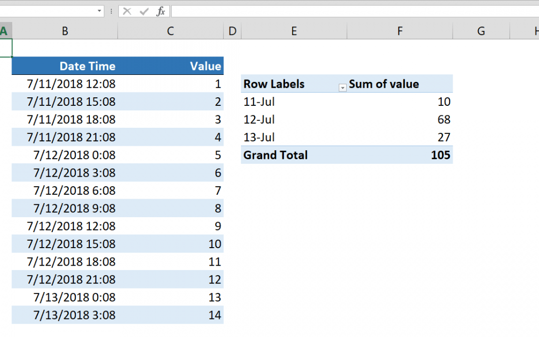
Excel already has functions like the SUMIF and the SUMIFS for summing data by groups. However, they won't work when have date-time values combined. In this article we will cover grouping dates in Pivot Table.
Steps
- Select a cell in your data
- Click Pivot Table icon under INSERT tab in the ribbon
- Confirm the data range and the location of the Pivot Table
- Click OK to create
- Drag & drop the date values into ROWS section and values into VALUES section
- Right-click on the date value in Pivot Table and click on Group item
- Select only Days
- Click OK to group
How
The Pivot Table is a versatile tool that specialized on data management and consolidation. As well as you can get consolidated data just by dragging & dropping column names into related sections, it offers advanced and detailed grouping options. Grouping dates in Pivot Tables can be done by years, quarters, months, days, hours, minutes and even seconds.
Another advantage of Pivot Table is its consolidation options. Using formulas to make similar grouping will restrict you on sum or count operations. However, Pivot Table allows to summarize values by Multiplying to Standard Deviation.
Also refer to article How to group days without time by formula


