It’s often a good idea to highlight the duplicate values in a data set to help easily identify the outliers. Let us show you how to highlight values based on item lists using Conditional Formatting.

Syntax

=COUNTIF( absolute reference of list of values, relative reference of the first cell in highlight range)

Steps

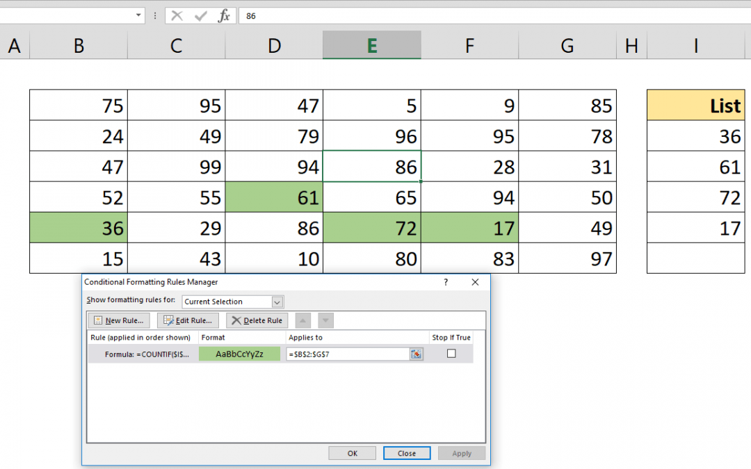
1. Begin by selecting the data range (i.e. B2:G7)
2. Open the Conditional Formatting window by going to HOME > Conditional Formatting > Add New Rule
3. Select Use a formula to determine which cells to format
4. Enter the formula that compares the first cell with COUNTIF function =COUNTIF($I$3:$I$7,B2)
5. Click the Format button to edit formatting settings
6. Click OK to continue and apply your settings

 How

The conditional formatting feature applies selected formatting options to a cell, when a given condition is met. If this condition is provided by a formula, Excel will check whether the formula returns TRUE before applying formatting options. Therefore, we need a formula that will return TRUE when the value in a cell occurs more than once within the selected range.

The COUNTIF function returns the number of cells that meets specified criteria. So, the idea is to check the cell count to see whether there are any items that repeat more than '0' times. Excel assumes all whole numbers are equal to TRUE, except for '0'.  If the result is TRUE, we want it highlighted. The COUNTIF function takes two arguments (range of values, and the criteria) to specify which values to return. For example,

=COUNTIF($I$3:$I$7,B2)

Fortunately, we do not need to add conditional formatting to each cell one-by-one. Excel can handle this by looking at absolute and relative references. All you need to do is to make an absolute range reference (i.e. $I$3:$I$7) for your list because the list should be the same reference and leave the first cell (i.e. B2) relative. This way, the range can be updated for other cells to be added.

Also see our How to highlight to find out about other cell highlighting options.