
Quartiles play a crucial role in statistical analysis, providing insights into data distribution. Excel's Quartile functions, including QUARTILE.INC, empowers users to calculate these significant points efficiently. In this comprehensive guide, we delve into understanding quartiles, using Excel's quartile functions and dynamically highlighting them using Conditional Formatting.
Unraveling the Basics
Before delving into the application of quartiles in Excel, it's essential to comprehend their significance. Quartiles divide a dataset into four equal parts, offering a nuanced view of its distribution. Excel facilitates this analysis with the QUARTILE.INC function, taking in the data array and quartile number as parameters.
The quartile numbers (0 to 4) correspond to specific percentiles, delineating the dataset as follows:
- 0: Minimum value
- 1: First quartile (25th percentile)
- 2: Median value (50th percentile)
- 3: Third quartile (75th percentile)
- 4: Maximum value
Excel Quartile Function: Mastering the Syntax
The QUARTILE.INC function syntax is crucial for accurate implementation. Using a relative reference for the first cell, the formula dynamically identifies the quartile category of each value. Let's break down the formula:
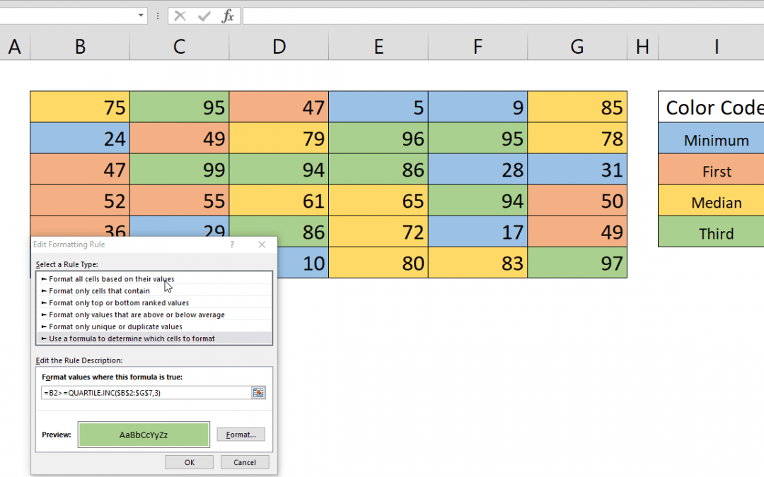
=B2>=QUARTILE.INC($B$2:$G$7,3)This formula checks if the value in cell B2 is greater than or equal to the third quartile (75th percentile) of the dataset in the range B2:G7. By applying this formula across the dataset, we can dynamically highlight values based on their quartile category.
Highlighting Quartiles with Conditional Formatting
- Select Data Range: Select the dataset range (e.g., B2:G7).
- Open Conditional Formatting Window: Navigate to HOME > Conditional Formatting > Add New Rule.
- Use a Formula: Choose "Use a formula to determine which cells to format."
- Enter Quartile Formula: Input the quartile formula for the first cell, such as
=B2>=QUARTILE.INC($B$2:$G$7,3). - Edit Formatting Settings: Click the Format button to customize formatting options.
- Apply Settings: Confirm and apply the settings by clicking OK.
Behind the Scenes
Conditional Formatting dynamically applies formatting based on the formula's conditions. In this case, the formula compares each cell's value with the third quartile limit. If TRUE, the formatting is applied. Leveraging absolute and relative references ensures that the range adapts as new cells are added.
Additional Applications
Excel's Conditional Formatting is a versatile tool. While we've focused on quartiles, this technique can be adapted for various scenarios. Explore other articles to discover innovative ways to leverage Conditional Formatting for data analysis and visualization.
Mastering quartiles in Excel, coupled with dynamic highlighting through Conditional Formatting, empowers users to gain deeper insights into their datasets. Understanding the quartile function's syntax and applying it judiciously opens the door to advanced data analysis in Excel. As you explore these techniques, you'll find many possibilities for enhancing your data interpretation skills.
For further insights and advanced applications of Conditional Formatting, refer to the link to access a diverse range of articles. Elevate your Excel proficiency and unlock new dimensions of data analysis with these valuable resources.