Using different coloring makes it easy to highlight differences in data or the layout of your spreadsheets. Excel has support for rows with alternating coloring in tables. What if your table contains similar values in groups, and you want to color the rows based on these groupings? In this guide, we’re going to show you how to alternate row color based on group in Excel.
If you are only interested in creating rows with alternating colors, you have two options:
- Convert your table into an Excel Table. See how you can create an Excel Table.
- Apply conditional formatting for each row: How to highlight alternate rows in Excel
Data
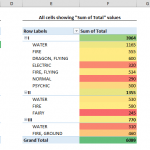
The following table is our sample data. Note that the Generation column contains values in three groups. Our aim is to assign colors into each group.

First step is to create a helper column to return a different value when the group is changed. The helper column will be the source for the conditional formatting.
- Start by adding a new column into your table.
- Type in 0 (zero) for its title. This is only necessary for the first cell.
- Add the following formula into the helper column and make sure to copy down for the rest of the rows. Remember to update cell references accordingly.

The function generates 0 and 1 with the MOD function. The next step will be to add the conditional formatting to color the rows by 0 and 1.
Conditional formatting to alternate row color based on group
In a nutshell, conditional formatting can apply formatting to a cell based on a condition. Let’s see how you can apply this to your table.
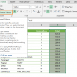
- Start by selecting the data and ignore the header row.
- Follow the path in the Ribbon: Home > Conditional Formatting > New Rule

- Select Use a formula to determine which cells to format option. Other options work for the value of each cell.
- Enter a formula and include the reference of the first cell of the helper column with a =1 (equals to 1) notation. This formula will return a logical value, TRUE or FALSE based on the cell’s value. Formatting will be applied if the value is TRUE.
- Click the Format button to open Format Cells

- To apply a background color, activate Fill
- Select a color.
- Click OK on each window to save.


Here is the result:

Tips and Remarks
Condition Formatting Formula
It is very important to lock column the references in the conditional formatting formula. Locking means to putting a dollar sign ($) in front of the column or row identifier when referencing them. By locking, the column and/or the row will not change when copying the formulas.
The same behavior applies to conditional formatted ranges as well. By putting a “$” in front of the column reference, you ensure that the formula always look at that column. To learn more about locked/unlocked references, you can visit our guide.
More colors
You can add conditional formatting for each value in the helper column. For example, to make a 2-color version, follow the same steps by using the following formula with a different color: