Calculating averages by week number is a bit different than doing this by month. Instead of finding start and end dates of date range, we focus on the exact week number using the WEEKNUM function.
Syntax
=AVERAGEIFS( range of values to calculate average, range of week number helper column, current week)
Steps
- Add a helper column near your table
- On the helper column, use WEEKNUM function with actual dates =WEEKNUM(B3)
- Go to results table with week numbers
- Start with =AVERAGEIFS(
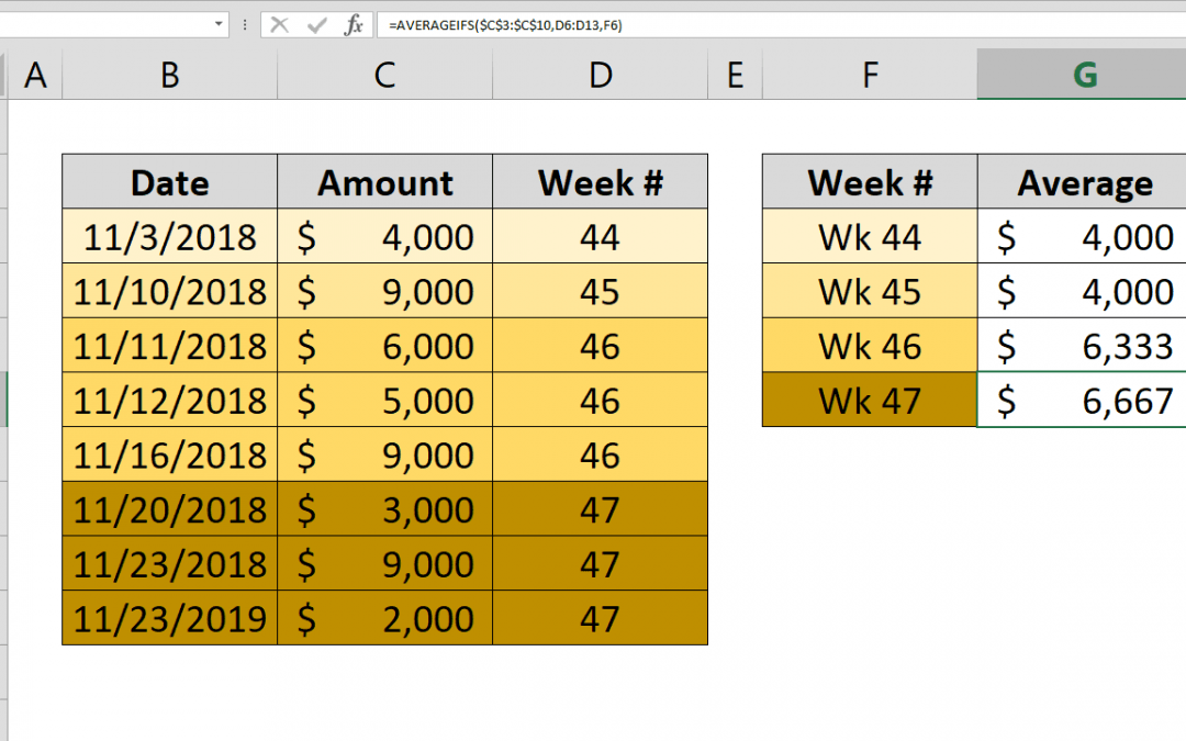
- Select or type in the range reference that includes the calculated values (i.e. $C$3:$C$10,)
- Continue with 'criteria range' – 'criteria' pair with week range and week number for the first row (i.e. $D$3:$D$10,F3)
- Type in ) to close the SUMIFS function and press Enter to complete the formula
How
The AVERAGEIFS function calculates averages for cells that meet any given criteria. Instead of filtering dates in a month, we get help from the WEEKNUM function which returns the week number of a specified date. So, first step is to add a helper column to convert actual dates to week numbers.
=WEEKNUM(B3)
From here on, we can use AVERAGEIFS (or even the AVERAGEIF formula because we have only one criteria, week number) to calculate the average. The AVERAGEIFS first argument is the values to sum. Other arguments are the 'criteria range' – 'criteria' pairs. Since we have single criteria, we use 3 arguments.
=AVERAGEIFS($C$3:$C$10,$D$3:$D$10,F3)
Please pay attention to absolute references on values and criteria range. They should remain same as we copy down our formula from week 44 to 47. The Criteria argument has relative reference because we want it to be updated through rows.
We can display week numbers with a "Wk" perfix. Adding custom format "Wk 0" to a number adds "Wk" text at front of number. To apply a custom format:
- Select the cell to be formatted and press Ctrl+1 to open the Format Cells dialog. An alternative way to do is by right-clicking the cell and then going to Format Cells > Number Tab.
- Under Category, select Custom.
- Type in the format code into the Type
- Finally, click OK to save your changes.
For detailed information about Number Formatting please see: Number Formatting in Excel – All You Need to Know