In finance, understanding option pricing is important for accurately estimating the value of option contracts based on all available data. Utilizing tools like Excel and Monte Carlo simulation, you can effectively simulate a wide range of scenarios. This guide will show you how to do a Monte Carlo simulation in Excel, specifically tailored for option pricing. By leveraging Excel's features, such as the Monte Carlo Excel add-in and Monte Carlo simulation Excel templates, we will explore how to run Monte Carlo simulation and employ probability formulas in Excel. This approach enhances the accuracy of your financial models and equips you with the skills to conduct comprehensive what-if analysis and Monte Carlo analysis in Excel for various financial scenarios.
What is Monte Carlo Simulation?
Monte Carlo simulation, a key method in Excel simulation, stands out as a distinct probability Excel tool primarily utilized to assess risk by analyzing a spectrum of potential outcomes. Originally devised to predict the various endings of a solitaire game, the Monte Carlo method derives its name from the renowned casino hub in Monaco, reflecting its probabilistic foundations.
This technique in Monte Carlo simulation in Excel involves assigning random values to variables within specified boundaries, a key feature in Excel probability functions. As the Monte Carlo Excel add-in runs more iterations, a comprehensive pool of results emerges, crafted from these varied inputs.
This approach is particularly effective in financial modeling, such as simulating future stock prices in Excel. By leveraging Monte Carlo simulation Excel templates, we can forecast stock price trajectories and subsequently calculate the discounted expected payoffs of options, integrating the core principles of Monte Carlo analysis in Excel. This method not only enhances the depth of financial analysis but also aligns perfectly with the requirements of running Monte Carlo simulations in Excel for diverse financial scenarios.
Leveraging Excel's powerful statistical function, NORM.S.INV, and Visual Basic for Applications (VBA), we can create random variables that follow a normal distribution. This combination is crucial for efficiently conducting Monte Carlo simulation in Excel. By harnessing these tools, we can simulate scenarios multiple times, a vital step in ensuring the robustness and reliability of our Monte Carlo analysis in Excel. This approach aligns with the principles of Excel simulation and optimizes the process of running Monte Carlo simulations in Excel, making it an indispensable technique for advanced financial modeling and probability calculations in Excel.
European-style Options Pricing
In our demonstration, we'll apply the renowned Black-Scholes formula, a cornerstone in financial modeling, to compute the pricing of a European-style option. This model is characterized by its restriction on exercising the option only at its expiration date. Within the realm of options, there are primarily two categories: call options and put options. Each type represents a different strategy and outcome in financial decision-making, and understanding these is crucial when running Monte Carlo simulations in Excel for option pricing analysis.
- A Call option represents a contractual agreement between the buyer and the seller, where the buyer is granted the right, but not the obligation, to purchase a specified security at a predetermined price. This type of contract plays a critical role in financial strategies and is a key element to understand when conducting Monte Carlo simulations in Excel for option pricing.
- A Put option is a type of contract that grants the holder the right, but not the obligation, to sell a particular asset at a predetermined price within a specified timeframe to the seller of the put. This financial instrument is essential in portfolio management and is a crucial concept in Monte Carlo simulations in Excel, especially when analyzing different market scenarios and option pricing strategies.
The Black-Scholes formula is widely acclaimed for its effectiveness in determining the value of European call-and-put options. At its core, this formula considers two principal factors: the risk-free rate of return and the volatile nature of stock prices. The model provides a fundamental equation that illustrates the fluctuation of stock prices over time, offering a clear perspective on how these variables interact in the context of option pricing. This formula is especially relevant in Excel's Monte Carlo simulation, which is a foundation for analyzing and predicting option values under varying market conditions.

In our Monte Carlo simulation within Excel, we focus on several key variables to accurately model stock price movements over time. Here's a breakdown of these critical elements:
- St: This represents the stock price at a specific time 't'. It's a dynamic value, changing with market conditions and time, and is central to our simulation.
- r: The risk-free rate, which is a theoretical return on an investment with no risk of financial loss. In financial models, this rate is crucial for discounting future cash flows to their present value.
- t: Time, typically measured in years, is an essential factor in option pricing models. It impacts the value of options as they approach their expiration date.
- σ: This denotes the volatility of the stock's returns, calculated as the square root of the stock's log price process's quadratic variation. High volatility increases the potential range of future stock prices, which is a vital consideration in option valuation.
- ε: A randomly generated variable following a normal distribution, crucial for introducing randomness into the Monte Carlo simulation, mimicking real-world stock price movements.
- δ: The dividend yield, which was not included in the original Black-Scholes model. The initial model was developed for options on stocks that do not pay dividends. However, including dividend yield allows for a more comprehensive analysis in modern applications.
After running the formula through thousands or millions of iterations in the Monte Carlo simulation Excel, we compile a set of St values, reflecting the potential future prices of the stock. To determine the payoff values, we then apply another formula where K represents the strike price of the option. This process allows us to estimate the option's value under a wide range of possible future scenarios, making it a powerful tool for financial analysis and decision-making.


Calculating Option Pricing with VBA
Next, we'll integrate these formulas into a custom VBA script. We aim to develop a user-defined function (UDF) like Excel's native functions, such as SUM or VLOOKUP. This custom function, which we'll name 'EuropeanOptionMonteCarlo,' is designed to harness the power of the Monte Carlo simulation directly within Excel. This approach streamlines the process of option pricing analysis and enhances the flexibility and efficiency of using Excel for advanced financial modeling.
Public Function EuropeanOptionMonteCarlo(OptionType As String, S As Double, K As Double, r As Double, sigma As Double, T As Double, Div As Double, N As Double, nIt As Double)
Dim i As Integer, j As Integer
Dim Payoff() As Double, St As Double, dt As Double, e As Double, price As Double
ReDim Payoff(1 To nIt)
dt = T / N
Randomize 'new seed for random number generation
For i = 1 To nIt
St = S
For j = 1 To N
e = WorksheetFunction.NormSInv(Rnd()) 'random factor
St = St * Exp((r - Div - sigma ^ 2 / 2) * dt + sigma * Sqr(dt) * e) 'European option formula
Next j
If OptionType = "Call" Then 'Call or Put
Payoff(i) = WorksheetFunction.Max(St - K, 0) * Exp(-r * T)
ElseIf OptionType = "Put" Then
Payoff(i) = WorksheetFunction.Max(K - St, 0) * Exp(-r * T)
End If
Next i
For i = 1 To nIt
price = price + Payoff(i) 'Total of iterations
Next i
EuropeanOptionMonteCarlo = price / nIt 'Return average of iterations as the function's result
End Function
Once the UDF is ready, we are ready to see the result in Excel.