A final exam is worth more in terms of graduation score and the term weighed average becomes relevant. In such cases, SUMPRODUCT formula can help calculate the weighed totals of a data set.
In our example, test scores of 3 candidates are being compared. Although Candidate 1 has higher scores according to standard average of scores, Candidate 2 actually has the lead by weighted average and comes at the first place.
Syntax
=SUMPRODUCT(weights array, actual values array) / SUM(weights array)
Steps
- Type =SUMPRODUCT(
- Select or type in the range reference that includes weights $C$3:$C$7,
- Select or type in the range reference that includes scores D3:D7)
- Use a slash ( / ) to divide total number to sum of weights
- Continue with SUM(
- Select or type in the range reference that includes weights $C$3:$C$7
- Type ) and press Enter to complete formula
Tip: If you have a table similar to this, make sure to make the "weight array" absolute ($C$3:$C$7) and "values array" relative (D3:D7) in order to populate ranges. You can change absolute/relative status of a range by pressing F4 key while your cursor is on it.
How
Weighed average of values are calculated by multiplying actual values by a weight factor and dividing the sum of these values by the sum of their weight factors.
Instead of multiplying each value by its corresponding weight in an additional helper column and sum them, SUMPRODUCT function can directly make this calculation inside a single cell. Last step is to divide the total value to sum of weight factors.
Note: Because the weight factors in our example add up to 100%, it may seem unnecessary to do the last division. However; weight factors can be regular numbers (i.e. 1, 2, 3) that add up to a 10 for example. In this case, skipping the division will provide the wrong result.


