The logical tests and conditional checks have important role in Excel models. Potential errors can be detected and handled by using the right logical tests. If you know How to check if a value exists in a list, you can use this logical statement to detect and eliminate erroneous scenarios.
Syntax
=COUNTIF(list, search value)>0
=NOT(ISERROR(MATCH(search value, list, 0)))
Steps
- Start with =COUNTIF( function
- Select or type the reference that contains the list range $C$3:$C$27,
- Select or type the reference that contains the value E4
- Type ) to close the COUNTIF function
- Type >0 to add the conditional check and complete the formula
How
There are more than one way to check if a value exists in a list or a range as well. You can count the value by COUNTIF, COUNTIFS or even SUMPRODUCT functions or check its position in an array with MATCH function. Although checking the existence of a value is not their main purpose, they can return a TRUE/FALSE values with some tweaks.
COUNTIF, COUNTIFS
Both functions can count a specific value in a given array. Because we only need to count a single value, COUNTIFS shares the same syntax with COUNTIF. Both functions uses a criteria range-criteria pair for their first two arguments. They return a numeric value greater than 0 if the value exists in an array and return 0 if the value doesn't exist.
=COUNTIF($C$3:$C$27,E4) returns 1
=COUNTIF($C$3:$C$27,E5) returns 0
By adding >0 condition, we can get a TRUE/FALSE value for exist/not exist condition respectively. Excel returns Boolean values as a result of logical statements.
=COUNTIF($C$3:$C$27,E4)>0 returns TRUE
=COUNTIF($C$3:$C$27,E5)>0 returns FALSE
MATCH
The MATCH function returns the position of a specified value in a one-dimensional range. It returns an integer when the value is found. Its arguments are the specified value, the range of data and 0 to ensure to search is based on exact match. However; it returns an error if there is no match. Because of this behavior, we need to check the error condition instead of the returned number.
=MATCH(E4,$C$3:$C$27,0) returns 25
=MATCH(E5,$C$3:$C$27,0) returns #N/A!
The ISERROR function can help to check if there is an error or not. It returns a Boolean value: TRUE if there is an error or FALSE if not. We have already handled the Boolean values with COUNTIF and COUNTIFS functions above. However; we have opposite situation in this case.
=ISERROR(MATCH(E4,$C$3:$C$27,0)) returns FALSE
=ISERROR(MATCH(E5,$C$3:$C$27,0)) returns TRUE
To reverse a Boolean value or the result of a logical statement, we can use the NOT function. The NOT function returns the opposite value of its Boolean argument.
=NOT(ISERROR(MATCH(E4,$C$3:$C$27,0))) returns TRUE
=NOT(ISERROR(MATCH(E5,$C$3:$C$27,0))) returns FALSE
SUMPRODUCT
The SUMPRODUCT function can be used as an alternative to these functions. It can be modified to return a similar value to COUNTIF and COUNTIFS. The SUMPRODUCT function can handle arrays without being an array formula. You can get the count of the value in an array based on a criteria range-criteria equality.
=SUMPRODUCT(N(C3:C27=E4))>0 returns TRUE
=SUMPRODUCT(N(C3:C27=E4))>0 returns FALSE
You can also see How to count values by length article.