In this article, we are going to show you how to consolidate text by a condition in Excel.
Please note that we will be using the new dynamic array functions UNIQUE and FILTER in this post. These functions currently are only available to Office 365 users.
If you don't have Office 365, a great alternative to these formulas is using a Pivot Table instead. To learn more about this method, please see How to consolidate text with Pivot Table in Excel.
Consolidating text by a condition
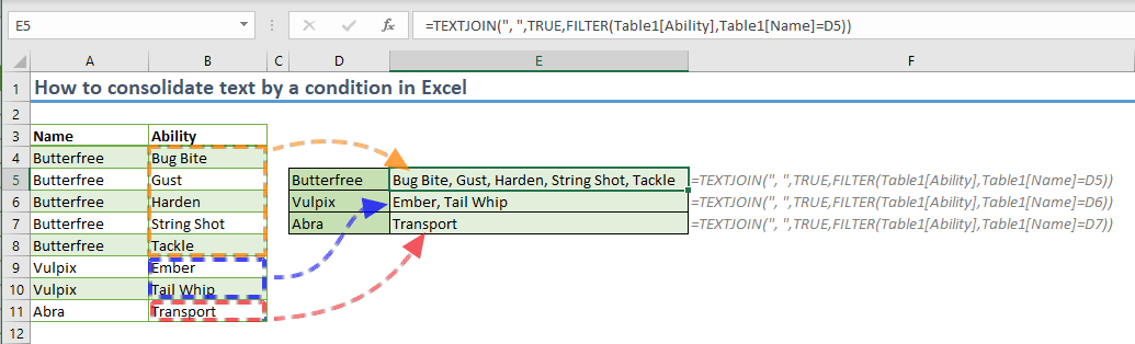
The example we are going to be looking at consists of categories (Name), and corresponding text values (Ability) we want to consolidate.
Note that you can convert your data into an Excel Table by pressing Ctrl + T when the data is selected. An Excel Table provides a dynamically updating table layout and makes formulas easier to apply. See Tips for Excel Tables for more.

First, we need a list of conditions (categories). This list needs to include unique names to avoid any duplicate entries. If you already have a list of conditions, you can use it as is.
You can generate a unique list using the UNIQUE function. Use the Name column to populate a list of unique categories.

Next, we can use these unique values to “filter”, and merge the values under the Ability column. The consolidation formula will include FILTER and TEXTJOIN functions.
In summary, the FILTER formula can return an array of values based on a criteria, and the TEXTJOIN can merge text values in an array, adding a delimiter.
The criteria in our scenario can be defined with the Table1[Name]=<Category> expression. So, replace <Category> with the reference of the unique Name value.
The first argument of the TEXTJOIN function determines the delimiter. Our choice is a comma and a space ", ". You can replace this with any value you want like “ - ", “ | “, etc.