In this article, we are going to show you how to consolidate text with Pivot Table in Excel 2013 or newer.
If you are using Office 365, also see our alternative approach for consolidating text in Excel. Thanks to the dynamic array functions like UNIQUE and FILTER, you can achieve the same result with a more dynamic approach.
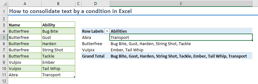
Consolidating text strings using Pivot Table
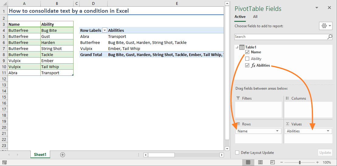
The example below contains category names (Name), and corresponding text values (Ability) we want to consolidate.

With a regular Pivot Table, you can easily group categories and consolidate numbers (see Pivot Table Alternative Using Formulas). You can't do this using formulas in a Pivot Table, but you can add this feature using DAX formulas.
To be able to use a DAX formula in a regular pivot table, you need to create a Data Model. Here are the steps:
- Click on your data.
- Follow Insert > Pivot Table > From Table/Range (this might look different based on your Excel version).

- Enable the Add this data to the Data Model checkbox in the PivotTable from range or table.
- Click OK to create a pivot table.

- Before adding fields into the pivot table area, you need to create the measure to be used in consolidating the text strings. Right-click on the table name in the PivotTable Fields pane and click Add Measure.

- Give the measure a name and enter the formula based on your data. Then, click OK to add the measure.

- Once the measure is ready, move the category field (Name) into Rows and new measure (Abilities in our sample) into Values. The pivot table will show the results.


How it works
The CONCATENATEX function is an updated version of the old CONCATENATE function. The DAX version can merge an array of strings with a given delimiter.
The DAX formulas also requires a table and column name as well. Thus, the syntax is the following:
Once the measure is ready, you can use it like any other pivot table field. The pivot table can group or filter the data, and also run the formula in the measure.