Although Excel doesn’t have a built-in feature to count cells by their colors, filtering cells by their color is possible. In this guide, we're going to show you how to count colored cells in Excel.
Steps
- Right-click on a colored cell in the data. Make sure to select the cell with the color you want to count.
- Click Filter > Filter by Selected Cells Color to filter the colored cells.

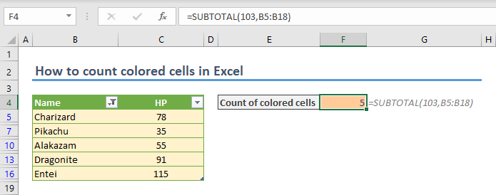
- Type in the following formula =SUBTOTAL(103,<data range>) where <data range> is the reference of your data. It is B5:B18 in our example.


How it works
The SUBTOTAL function can perform various aggregation operations with and without using manually hidden rows. In this example, Excel hides the rows with unwanted values when the filtering is applied. Thus, the filtered-out values remain in manually hidden rows. The SUBTOTAL function can exclude the values in the hidden rows. As a result, it can return the number of colored cells.
The SUBTOTAL function supports the capabilities of both COUNT and COUNTA. The function type is determined by the first argument. Choose either 102 or 103 for COUNT and COUNTA functionalities respectively.
The second argument is the range where you want to count cells.
Using a table to count colored cells
You can use this method if you keep your data in an Excel Table (which we recommend). You can add a total row and select the function from a dropdown menu.
- After converting your data into a table and filtering by color, select any cell in the column you want to count.
- Enable the Total Row checkbox in Table Design tab in the Ribbon.
- Click on the number added to the last row.
- Click on the arrow to see the options. Select Count.

Excel automatically adds a formula with the SUBTOTAL function. You do not need to relocate formula thanks to the dynamic structure of Excel Tables.