A stream graph is a form of stacked area chart in a flowing, organic shape. The graph is displaced around a central axis to visualize the data without expressing positive or negative values. In this guide, we’re going to show you how to create a stream graph in Excel.
At the time of writing this article, stream graphs are not supported in Excel natively. Because the stream graphs are derived from area charts, we are not out of options. Let's see the steps to create a stream graph in Excel.
Modifying the data before create a stream graph
The first step is to make your data suitable for a stream graph. Why? There are two reasons:
- A stream graph floats above the axis while an area chart fills entire area starting from the axis.
- Sharp lines between data points do not give the flowing impression.
How to make the data float
A regular area chart looks like the following.

To apply the floating effect, we need a dummy data which will be placed between the x-axis and the actual data. Once the dummy data is in the chart, we can use transparent color to hide it.
The dummy data should be calculated according to your actual data to be able to elevate it. This means that you need a big enough number which can lift at least the height of total area for each data point. You can either use a static value if you already know the maximum heights for each point or sum each data point for all categories and find the maximum value. Simple SUM and MAX functions can handle this easily.

Once the maximum height is calculated, use the number to create the numbers for floating data. Our choice is to subtract half the heights from the maximum height value and add a randomly generated number. Dividing the value by half is necessary to ensure not to lift actual values too much. A random variable is to add a natural look. The idea of generating a flowing graph is more important than precision for stream graph. You can use RANDBETWEEN function to generate random integers.
Feel free the change the formula to male it fit to your data and graph.

At this point, you can skip the smoothing step and create your stream chart right away. However, the sharp lines will prevent the flow effect.

How to create a smooth chart data
You may have been familiar with smoothed line charts already. However, area charts do not have this option. Thus, you should smooth the data yourself. In a nutshell, the data smoothing is a statistical approach to be used to help predict trends by trying to ignore outliers. The common methods of smoothing are moving averages, exponential smoothing, and linear regression. We have chosen the moving averages technique (the easiest) in this article. For more information, you can check out Forecasting in Excel article.
Moving averages is very simple technique to apply. All you need to do is to calculate the average of determined number of values including the corresponding data points. We have calculated averages for three numbers. For example, the fourth data point in the "HP" column will be equal to the average of second, third and fourth values (C6:C8). Use the AVERAGE function to calculate averages. You can skip the data points less than the number of points. For example, we have skipped the first and second numbers since we are averaging by three (3) point.

Once you are OK with smoothing, you can start creating your stream graph.
Creating a stream graph in Excel
Select your data and insert an area chart by following Insert > Insert Line or Area Chart > Stacked Area Chart path in the ribbon.

Once the chart is created, make sure that the Dummy data fills the area between horizontal axis and the data.

If not, right-click on the chart and click Select Data item to open Select Data Source dialog. Select the Dummy series in the left box and use the arrow buttons to place it on top.

After confirming the Dummy is at the bottom of the chart, right-click on the Dummy graph and select No Fill in the Fill menu to make the section transparent.

Use the Chart Elements button, the plus at top-right corner, to remove Gridlines. This action completes the floating effect.

Final step is to get rid of the Dummy item in the legend. Click on the label twice to select the dummy column only. Then press Delete button.

Preferably update or remove the chart title. You can remove the vertical axis as well since the exact values are not important.

Bonus
You may add dummy entries at the beginning and the end of your chart data to generate wrapping lines around your chart. Download the workbook to see exact calculations.