In this guide, we’re going to show you how to create a To-Do list in Excel with the help of checkbox controls and conditional formatting.
Preparation before creating a To-Do list
Start by creating a 3-column range for the to-do list. These columns can include:
- To-Do items
- Checkboxes for status
- Helper column for storing the values of checkboxes

Checkbox controls can go under the status column. You can add multiple checkboxes by creating one inside a cell and dragging it down for the rest.

See how to insert a checkbox in Excel for more details on how to add checkbox controls.
Once the checkboxes are ready, link them to adjacent cells under the Helper column.

Once linked, check and uncheck the checkboxes to make sure they are linked correctly. You will see that cells in the Helper column show either TRUE or FALSE value based on the checkbox selection.

Helper column is actually optional. Now, let's take a look on further customization options for our To-Do list.
Adding conditional formatting
Conditional formatting is great way to help distinguish completed and not-completed items.
- Select all of to-do items in your list.
- Open the New Formatting Rule window by following Home > Conditional Formatting > New Rule.

- Select Use a formula to determine … item in New Formatting Rule
- Enter a formula which is using the NOT function with the reference of the first cell of the Helper. Be sure to leave the row part relative: =NOT($D5) (Relative reference is important to let Excel copy the formula to other cells in the column).
This formula allows you to format unchecked items, because FALSE will become TRUE thanks to the NOT function. TRUE tells Excel to apply the determined format. - Click the Format button to open Format Cells
- We selected a grey font color and strikethrough font type to express completed items.
- Click OK buttons in all windows to apply the formatting.


Once the formatting is applied, you will see something like below.

If you are satisfied with the result, just hide the helper column and you're done. Next, we are going to place a progress indicator.
Progress
Since we are already keeping the values of checkboxes in the helper column, we can count them and calculate the ratio of checked items. The COUNTA and COUNTIF functions can help here.
If we name Helper column as "Helper", the formulas will be like below.

While the COUNTA function counts cells that contain a text, the COUNTIF function counts the cells containing only TRUE. The ratio between two gives us the progress.
You can also add a visualization to display this information. Although Excel doesn't have a visualization called "progress bar", you can create one by modifying a bar chart.
- Insert a bar chart by following Insert > Insert Column or Bar Chart > Clustered Bar (2-D Bar).

- Right-click on your chart area and click Select Data.
- Use Chart data range input to select the ratio.

- Click OK to see the chart. With a couple of visual modifications, this bar chart will become a progress bar.

- Double-click on the vertical axis to see the options. Open Axis Options and set Minimum to 0 and Maximum to 1.

- Remove the vertical axis.
- Remove the title.
- Shrink the area by decreasing the height.
- Add border to the Plot Area by right-clicking and setting Outline
- Decrease the Gap Width.