How to find all combinations of two lists in Excel

In this guide, we're going to show you how to find all combinations of two lists in Excel by using Power Query.

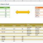
In our example, we have two lists that contain Pokémon names and we want to see the combinations of matched Pokémon.

We can join these two tables to compare them by using Get & Transform Data. Get & Transform Data feature consists of tools, previously known as Power Query. You can get more information about this here: Power Query 101.

Creating queries from tables

First step is to convert the tables into Power Query structure.

Select one of your tables.
Open the Data tab and click the corresponding icon under the Get & Transform Data section to get data from your workbook.
1. (Microsoft 365 / Excel 2019) From Sheet
2. (Excel 2016) From Table/Range
3. (Excel 2010 / Excel 2013) Use Power Pivot tab instead of Data
Clicking the button opens the Power Query Editor.
Once you are done with the changes, click Custom Column in Add Column. We will add a helper column which will be a common point between the two tables.
Enter a friendly name for your new column and enter =1 into the formula section.
Click OK to save.
After adding the helper column, return to the Home tab and click Close & Load To item in Close & Load list to see options.
Make sure to select Only Create Connection in the Import Data This option will save the table as a connection rather that populating the queried data in the worksheet.
Apply the same steps to the other table. At the end you should have two queries corresponding with your tables. You can see these tables in Queries & Connections pane in Excel.

Joining queries to find all combinations of two lists

Next step is to join (merge) the queries on a new table which will allow us to see any differences between the tables.

Once the queries from the tables are ready, go to Data > Get Data > Combine Queries > Merge to open the Merge dialog of Power Query.
Select each table in the drop downs.
Click on the column for each table to select them.
Finally select Full Outer option for Join Kind to join by all rows from both tables.
Click OK to apply selections.
You will see three columns after merging. The first one is the items of the first list. Right-click on the column in the middle and select Remove to delete the helper column.
Click the button next to the column title.
Make sure that the Expand option is selected in the popup menu.
Uncheck the helper column.
Uncheck Use original column as prefix.
Click OK to populate the data of the second table.
You will see the combinations in Power Query. When you are OK with the outcome, click Close & Load, this time to populate the entire data into your worksheet.