This article shows How to find closest match by using INDEX, MATCH, ABS and MIN functions. Excel's array formula ability to evaluate formula for each cells in an array is key factor in this case.
Syntax
{ =INDEX( return array,
MATCH(
MIN(ABS( search array – search value )),
ABS(search array – search value),
0
)
) }
Steps
- Start with INDEX function =INDEX(
- Enter the array reference that includes the data to return E3:E11,
- Continue with MATCH MATCH(
- Use MIN function for the first argument of MATCH MIN(
- Add ABS function to find absolute value of difference between search array and the value we search ABS(E3:E11-I3)
- Close MIN function and continue with next argument ),
- Once again add absolute value of difference between search array and the value we search ABS(E3:E11-I3),
- Use 0 for match type argument and close the functions 0))
- Press CTRL + SHIFT + ENTER instead of regular ENTER key to define formula as an array formula.
How
Closest Match = Minimum Difference
First of all, to find the closest match we should find the difference between the values in array and our search value. This means to make subtraction operation for each value in array. Because the closest means the close from both negative and positive direction, the difference values should be evaluated in same direction. The ABS function can help us in this matter by converting negative values to positive.
As a result, we need to get difference values between all values and search value in positive direction. Although, a helper column would be helpful in this, we can use array formula feature to complete all calculation in a single cell. So difference formula can be like this:
ABS(E3:E11-I3)
Normally, subtracting a value from an array returns a result only for the first cell of array. However, converting formula into an array formula enforces Excel to calculate for each cell. As a result, the formula returns
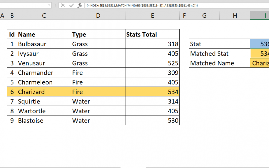
{218;131;11;227;131;2;222;131;6}.
Next step is to find the position of closest matched value. The MATCH function will do the hard work here. The logic is to find minimum difference (closest match) in an array of distances. There is nothing better than the MINIMUM function to find the minimum value in an array.
So, to find the position of the minimum difference, the formula will be:
MATCH(MIN(ABS(E3:E11-I3)),ABS(E3:E11-I3),0)
Return to basics: INDEX & MATCH
The rest of the formula is easy to figure out. It returns basic INDEX & MATCH combo that we have array of values and the position. To find the closest value, use the same array of values that is already used.
=INDEX(E3:E11,MATCH(MIN(ABS(E3:E11-I3)),ABS(E3:E11-I3),0))
Alternatively, you can select another related array, for example another column of the same table to return a value that is at the same row with matched value. For example; to get name from our sample table, we can use C3:C11 range that includes the names.
=INDEX(C3:C11,MATCH(MIN(ABS(E3:E11-I3)),ABS(E3:E11-I3),0))
The most important step is pressing CTRL + SHIFT + ENTER instead of regular ENTER key to define the formula as an array formula. Otherwise, you see #N/A error.