This article serves as your compass in navigating the seas of potential errors within your lists. We'll delve into a powerful strategy employing the ISERROR and MATCH functions within an array formula—unveiling a method to identify and manage errors in your Excel sheets systematically.
Understanding the ISERROR and MATCH Functions
Before we embark on the journey of error detection, let's acquaint ourselves with the ISERROR and MATCH functions. The ISERROR function checks if a particular cell contains an error, returning TRUE if an error is present and FALSE otherwise. On the other hand, the MATCH function locates the position of a specified value within a range.
Crafting the Array Formula
The synergy of ISERROR and MATCH comes to life when embedded within an array formula. This dynamic combination enables you to scrutinize an entire list efficiently, pinpointing cells harboring errors. The array formula extends the scope of your analysis, allowing for a comprehensive sweep through your data.
Detecting Errors in Your Excel Lists
The array formula makes identifying errors in your Excel lists a straightforward task. The ISERROR and MATCH collaboration empowers you to locate discrepancies, ensuring data integrity and reliability swiftly.
Managing Errors with Precision
Not only does this method reveal the existence of errors, but it also equips you with the means to manage them effectively. Whether correcting erroneous entries or implementing preventive measures, you gain a newfound control over the quality of your Excel data.
Syntax
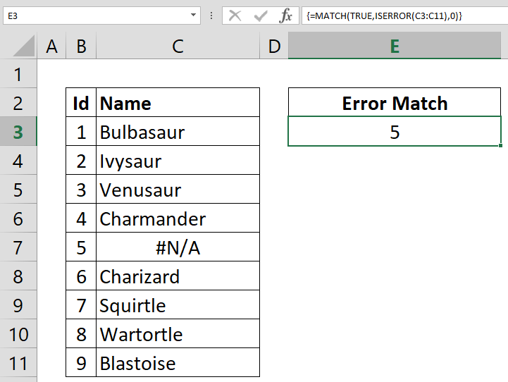
{ =MATCH(TRUE, ISERROR(search array), 0) }
Steps
- Start with =MATCH( function
- Type TRUE, variable to search for the matched values
- Continue with ISERROR( function
- Select the reference that contains the range to be searched C3:C11
- Type ) to close the ISERROR function
- Add 0 to ensure exact match
- Type ) to close the MATCH function and complete the formula
- Click Ctrl + Shift + Enter instead of Enter to make it an array formula
How to Find Errors
By default, you can't type an error in a formula and use it as an argument. Although #N/A error can be produced by the NA function, it can't be used. Because if there is an error in the function, the function also returns an error. Few functions can behave contrary to this assumption though. Functions like ISERROR or IFERROR accept errors as an argument. Also, some functions like COUNT or SUM ignore "only" #N/A errors.
We can use the ISERROR function to create an array and the MATCH function to locate the errors in the generated array. There are two tricks to apply here:
- Make the ISERROR function return an array handled automatically when we define it as an array formula.
- Search TRUE values, instead of the search value itself, in the array that is returned by the ISERROR function
Let's analyze the formula.
ISERROR(C3:C11) formula returns {FALSE;FALSE;FALSE;FALSE;TRUE;FALSE;FALSE;FALSE;FALSE} array for the list where the 5th value is an error. By defining the formula as an array we ensured the evaluation of the ISERROR function for each cell in C3:C11 range.
It is now straightforward to find the exact match using the MATCH function among TRUE/FALSE values.
=MATCH(TRUE,ISERROR(C3:C11),0)
Mastering the art of finding errors in your Excel lists transforms data management into a seamless process. The combination of ISERROR and MATCH functions within an array formula provides a powerful toolkit for identifying and addressing errors systematically. Embrace this strategy, and you'll not only enhance the accuracy of your data but also gain confidence in your ability to navigate the complex landscape of Excel errors.