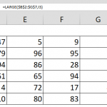
This article shows how to find largest value in array using LARGE and IF functions in an array formula.

Syntax

{=LARGE(IF(criteria range = criteria, data range reference), nth)}

Steps

1. Start with =LARGE( function
2. Continue with IF( to apply condition
3. Type the criteria range-criteria equation $E$3:$E$10=C$13,
4. Select the range that contains the data range $H$3:$H$10)
5. Type ) to close the IF function
6. Select cell that contains nth value or you can manually enter the value $B14
7. Type ) to finish and complete the formula.

How

The LARGE function returns the nth largest value in an array. We can modify the array by using the IF function that provides a logical test. In normal circumstances, logical test between a range and a value (or a cell that contains a value) returns a #VALUE! error.

$E$3:$E$10=C$13

To make this test work, the formula should be defined as an array formula and this can be done by pressing Ctrl + Shift + Enter keys instead of usual Enter. Ctrl + Shift + Enter combination "automatically" adds curly brackets around the formula. Please note that, you shouldn't type brackets manually. Once it is defined as an array formula, logical test will return an array of TRUE/FALSE values.

$E$3:$E$10=C$13 returns {TRUE;FALSE;FALSE;TRUE;FALSE;TRUE;TRUE;TRUE}

The IF function can then use the TRUE/FALSE values and return numerical values for TRUE items. There will still be FALSE items in the return array. The LARGE function ignores them and only evaluates the numbers.

IF($E$3:$E$10=C$13,$H$3:$H$10) returns {48972;FALSE;FALSE;44000;FALSE;87633;80850;80784}

Finally, the LARGE function will find largest value in array.

=LARGE(IF($E$3:$E$10=C$13,$H$3:$H$10),$B14)

Also see relevant articles how to find nth largest value in a data table, and how to find nth smallest value in a data table.