Excel has the MAX, MAXA and MAXIFS functions that can find the maximum value in a range or array. If you need to the position of the maximum value, however, you need to combine these formulas with others. In this article, we are going to show you how to find the position of the maximum value in Excel.
You may want to find the location of the maximum value, especially if you want to find other relevant values in the same row. Once you get the location, you can use the INDEX function incorporate that location as a coordinate. Let us see how you can find the position of the maximum value in Excel.
Single maximum value
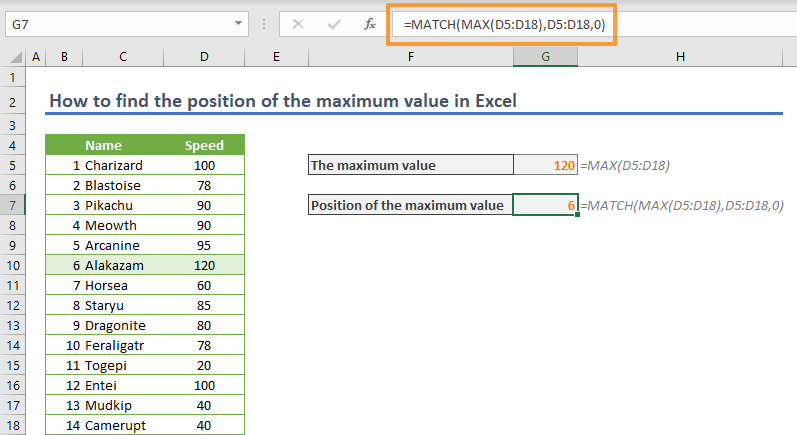
This is the most straightforward approach to locating the maximum value. The MAX function returns the maximum value in the range and the MATCH function returns the position of the maximum value in the given range.
In the following example, there is a list of names and numbers. The formula locates the maximum value in the Speed column, 120, and returns its position with the help of the MATCH function.
An important thing to consider is to remember to add 0 as the last argument of the MATCH function. The 0 value is a predefined value that runs the MATCH function in the exact match mode. To learn more about the MATCH function and its modes, see: Function: Match.
The negative side of this approach is that the MATCH function stops working when it finds the first suitable value. If your list contains the same maximum value multiple times, you cannot work with this formula.

Multiple maximum value
If we remove the Alakazam row from our table, the maximum value in the Speed column is reduced to 100. On the other hand, there are two 100 in the Speed column. As a result, we need to find the position of each occurrence of the maximum value.

Before continuing, please note that this approach is uses the dynamic array function FILTER. The dynamic array functions are available only for Microsoft 365 subscribers.
Briefly, the dynamic array approach can populate results into cells automatically and removes the need of using array formulas.
This formula uses the FILTER function to return the positions of the maximum values in a range. The first argument of the FILTER function includes the ROW function to generate the positions.
ROW(<range>) gives an array of the row numbers for the cells in the range. Subtracting ROW(<first cell of the range>) from the row numbers and adding 1 ensures an array of positions starting from 1.
The second argument of the FILTER function generates an array of Boolean values, TRUE and FALSE. This array makes the FILTER function include values with TRUE and ignore the rest.