You can find the minimum value in a range or array using the MIN, MINA and MINIFS functions. If you need to find the position of the minimum value instead, you will need a combination of these functions. In this article, we are going to show you how to find the position of the minimum value in Excel.
You may want to find the location of the minimum value, especially when looking for relevant values that appear in the same row as that value. Once you get the location, you can use the INDEX function incorporate that location as a coordinate. Let us see the methods for finding the position of the minimum value in Excel.
Single minimum value
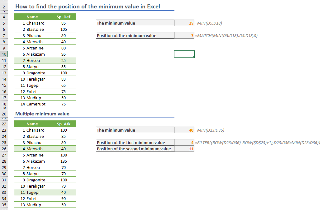
This is the most straightforward approach for locating the minimum value. The MIN function returns the minimum value in the range and the MATCH function returns the position of the minimum value in the given range.
In the following example, there is a list of names and numbers. The formula locates the minimum value in the Sp. Def column (25) and returns its position (7) with the help of the MATCH function.

An important thing to consider is to remember adding 0 as the last argument of the MATCH function. The 0 value is a predefined value for Excel which runs the MATCH function in the exact match mode. To learn more about the MATCH function and its modes, visit the function article: Function: Match.
The negative side of this approach is that the MATCH function stops working when it finds the first suitable value. If your list contains the same minimum value multiple times, you cannot work with this formula.
Multiple minimum value
Let us check Sp. Atk numbers which include same minimum number for 2 items: Meowth and Togepi. Either item has value of 40. Thus, you need to find the positions for each item.

Before continuing, we need to warn you that the following approach is using the dynamic array function FILTER. The dynamic array functions are available only for Microsoft 365 subscribers.
Briefly, the dynamic array approach allows populating results into cells automatically and removes the need to use array formulas.
This formula uses the FILTER function to return the positions of the minimum values in a range. The first argument of the FILTER function includes the ROW function to generate the positions.
ROW(<range>) gives an array of the row numbers for the cells in the range. Subtracting ROW(<first cell of the range>) from the row numbers and adding 1 ensures an array of positions starting from 1.
The second argument of the FILTER function generates an array of Boolean values, TRUE and FALSE. This array tells the FILTER function to include values coming across with TRUE and ignores the rest.