In this guide, we're going to show you how to flip data in Excel.
Using helper column And Sort feature
Our first approach is based on using a helper column and the Sort feature. This is a quick and dirty way to flip your data in Excel. The helper will order the values sorted by the Sort formula. For example, if the helper column has numbers from 1 to 5 in ascending order, sorting these numbers in descending order will reverse the values.
The Sort feature can be used to sort data according to the values in the helper column.
- Start by creating a helper column adjacent to your data.
- Click Sort in Data tab of the Ribbon.
- Make sure the helper column is selected in the Column
- Select the Order according to the numbers in the helper column. We selected Largest to Smallest because our numbers are in ascending order.
- Click OK to flip your data.


This is the flipped data. You can delete the helper column when you are done.

Flipping data with the SORTBY function
If you want a more dynamic solution, you can use the SORTBY, the SEQUENCE and ROWS functions.
Please note that the SORTBY, the SEQUENCE functions are currently only available only for Microsoft 365 users. If you are not a subscriber, you can check the next approach which involves using the INDEX function.
The SORTBY function can sort an array based on values in a corresponding array. This is similar to what the Sort feature does. The SEQUENCE and the ROWS functions provide the ordered values like the helper column.
The SEQUENCE function generates an array of numbers in descending order. The ROWS function’s goal is to provide how may numbers need to be generated. Although you can provide this information manually, we are using the ROWS function in this example for a more dynamic approach.

Using INDEX function as an alternative
Here is an alternative way if you don't have access to dynamic array functions like the SORTBY and the SEQUENCE. You can use the INDEX function with ROWS function to flip the data.
The INDEX function can return a value in an array based on the given row-column position. Thus, you can use the INDEX function with descending row or column numbers to list data starting from the end. For example, in our example each column has 6 rows. As a result, to return the last item first, the row argument should be 6 and go to 1.
To return the numbers in descending order, the ROWS function can be used. However, this time we will need collapsing (or expanding), meaning a range reference that uses relative and absolute references at the same time (e.g. B27:B$32). When this reference is copied to the cell below, it will become B28:B$32. Only the relative references will change while absolute remain as is. See our brief guide about absolute and relative references for more details.
We used separate formulas for each column to keep it simple. You can always add the column argument as well.