Number Formatting feature in Excel allows modifying the appearance of cell values, without changing their actual values. Currency formatting with dollar signs ($), or highlighting negative values with red are common examples. Another advantage of this feature is the ability to add thousands separators without changing the cell values. In this article, we're going to show you how to format numbers in Excel with thousands separators.
How
Number Formatting is a versatile feature that comes with various predefined format types. You can also create your own structure using a code. If you would like to format numbers in thousands, you need to use thousands separator in the format code with a proper number placeholder. For example; 0, represents any number with the first thousands part hidden.
42,000 will be displayed as 42
Here are some common placeholders:
|
Placeholder |
Description |
|
|
# |
Placeholder for digits (numbers) and does not add any leading zeroes. |
|
|
0 |
Placeholder for digits (numbers) and add any leading zeroes. |
|
|
. |
Placeholder for the decimal place. |
|
|
, |
Thousands separator |
Below are some examples:

Steps
- Select the cells you want format.
- Press Ctrl+1 or right click and choose Format Cells… to open the Format Cells dialog.
- Go to theNumber tab (it is the default tab if you haven't opened before).
- Select Custom in the Category list.
- Type in #,##0.0, "K" to display 1,500,800 as 1,500.8 K.
- Click OK to apply formatting.
Check out our detailed article for more information about Number Formatting: Number Formatting in Excel – All You Need to Know