This article shows how to get last match by using MAX, MIN, IF and ROW functions. Excel's array formula ability to evaluate formula for each cells in an array is key factor in this case.
Syntax
{ =MAX( IF( data = search value, ROW( data ) - MIN( ROW( data ) ) + 1 ) ) }
Steps
- Start with MAX function =MAX(
- Continue with IF function IF(
- Enter the match condition by using whole data range in an equation E3:E11=I3,
- Continue to next argument with ROW function and data range again ROW(E3:E11)
- Subtract following by previous step -MIN(ROW(E3:E11))
- Add 1 to calculation +1
- Close both formulas ))
- Press CTRL + SHIFT + ENTER instead of regular ENTER key to define formula as an array formula.
How
The logic is to find the maximum row number of the last occurrence of a match. Certainly, the finding maximum part is the easy part that Excel already has the MAX formula which can do the job without effort. So, let's check the remaining.
Relative Row Numbers
First of all; we need relative row numbers of data array that we can use it with the condition. The ROW function can easily give the row numbers of a range. When we use it in an array formula, it returns an array that includes the row numbers of each cell. To find the relative row numbers, we need to subtract first row of the range by row values of each cell. Also, adding 1 ensures that the row numbers start from 1.
ROW(E3:E11) returns {3;4;5;6;7;8;9;10;11}
MIN(ROW(E3:E11)) returns 3
As a result; ROW(E3:E11)-MIN(ROW(E3:E11))+1 returns {1;2;3;4;5;6;7;8;9}
Condition
Next, we use the array of relative row numbers with the IF function which has a condition for search value. Simple equation condition can do the job. Because we will use array formula, it is OK to use a range and a cell in equation. The array formula structure forces Excel to make calculations for each cell in the range. Here is the result for equation:
E3:E11=I3 returns {FALSE;TRUE;FALSE;FALSE;TRUE;FALSE;FALSE;TRUE;FALSE}
Combining TRUE/FALSE Boolean values with the row numbers returns the row numbers that condition is met.
IF(E3:E11=I3,ROW(E3:E11)-MIN(ROW(E3:E11))+1) returns {FALSE;2;FALSE;FALSE;5;FALSE;FALSE;8;FALSE}
Position
Finally, we can return to the MAX function. The MAX function evaluates Boolean values as 1 and 0 for TRUE and FALSE respectively. So, FALSE values are nothing in a MAX formula with positive numbers. The highest number indicates the position of the latest occurrence of search value.
=MAX(IF(E3:E11=I3,ROW(E3:E11)-MIN(ROW(E3:E11))+1))
Above all, the most important step is to press CTRL + SHIFT + ENTER rather than regular ENTER key to define the formula as an array formula. Otherwise, you see number 1 as the result.
Alternative
You can apply same logic for horizontal list just by converting the ROW functions with the COLUMN. Hence, a sample formula looks like this:
=MAX(IF(E3:N3=I3,COLUMN(E3:N3)-MIN(COLUMN(E3:N3))+1))