This article shows you how to get the nth match with VLOOKUP formula. Unfortunately, Excel doesn't have a built-in function to find any value beyond the first match.
Syntax
Unique lookup value: =lookup value & COUNTIF(expanding range of lookup values, lookup value again)
=VLOOKUP(Unique lookup value, table we look for, column number of where data is, 0 or FALSE for exact match)
Steps
- Add a new column to the left of your table and select its first cell
- Type the formula that generates a unique value =E3&COUNTIF($E$3:E3,E3)
- Copy down the formula to entire table column
- Use unique values in the new column, to get nth match with VLOOKUP function
How
Because there is no built-in function in Excel to locate and get the nth match, we are stuck with our dependable old friend VLOOKUP with a tiny tweak. As you know, VLOOKUP with FALSE argument will find the first exact match from a table. But you may have duplicate values hence multiple matches. So we need to create a helper column of unique values rather than bunch of the same values that is impossible to distinguish.
To achieve this, we will use COUNTIF function. Alternatively, COUNTIFS is also OK because we only need a single criteria and both work with same logic. The trick is to use an expanding range ($E$3:E3). The expanding range uses mixed references (absolute and relative) to expand from an anchor cell when you copy it down.
The COUNTIF function with an expanding range will create running count values with each row it is expanded. Merging the actual values -location names in our example- with running count numbers generates unique values (Gainesville1, Valdosta1, Valdosta2, etc.) that can be used with VLOOKUP.
=E3&COUNTIF($E$3:E3,E3)
The final step is to use VLOOKUP function as usual, but with unique values. But do not forget to merge the index number with actual lookup value before using the VLOOKUP.
=VLOOKUP("Valdosta"&G6,$B$3:$E$10,3,0)