Highlighting cells is a good way to visualize content and locate areas needing attention. Excel's Conditional Formatting feature is a great tool for this job. How to highlight cells by values article will show how you can create highlight cells based on different conditional statements.
Step by Step
- Begin by choosing the data range (B2:G7)
- Open the Conditional Formatting window by going to HOME > Conditional Formatting > Add New Rule
- Select Format only cells that contain
- Select the suitable condition from the dropdown
- Enter static values or cell references
- Click on the Format button to select the desired formatting options
- Click OK to continue and apply your settings
Conditional Formatting
Conditional formatting in Excel is a feature that allows users to dynamically format cells based on specified conditions, enhancing data visualization and analysis. When a given condition is met, the conditional formatting feature applies selected formatting options to a cell. Excel has built-in rules to cover most usage scenarios and a formula support to create user's own rules. If this condition is provided by a formula, Excel will check whether the formula returns TRUE before applying the formatting options. The Format-only cells that contain a rule are perfect for the conditions that check its value. You can set a rule to check if a cell's value is equal, between or not between the specified values, or even if a string starts with a certain string. To apply a rule that highlights cells by values "below 25", "between 25 and 75," and "above 75" differently, select Format only cells that contain the rule and select appropriate less than, between, and greater than conditions with desired colors. This will highlight cells by values based on selected rules.

Also, see related articles on how to highlight the top values in a data set dynamically and how to highlight duplicate values in a data set dynamically.
Mastering Excel's Conditional Formatting feature empowers you to visually pinpoint crucial data points efficiently. Following the steps, you can highlight cells based on specific conditions, tailoring your visual cues to different value ranges. Explore the versatility of conditional formatting to dynamically emphasize top values or identify duplicates, expanding your data analysis toolkit.
For in-depth guidance on Excel's conditional formatting, visit Microsoft's official documentation: Microsoft's Guide to Conditional Formatting.
As you delve into these techniques, you'll enhance your ability to extract meaningful insights from your data.