It is common to lose your way in a big table of data. Even though Excel's freezing features help you to display selected row and column's primary data, no feature can beat highlighting to express the selected data. In this guide, we’re going to show you how to highlight selected row and column in Excel.
Dynamic highlighting in Excel can be done by Conditional Formatting with ease. If you are not familiar with the conditional formatting, it is feature that allows you to change cells formatting based on a formula or value of cells.
You can apply the formatting into an entire row or column. However, Excel doesn't have a built-in function that returns the address of a selected cell. Thanks to VBA, we are not out of options. You can send the selected cell's row and column information to cells or named ranges by four-row code that you can either type or copy-paste. Follow the steps to highlight selected row and column in Excel.
1. Named ranges
Start by creating 2 named ranges. Named ranges allows you a simple formula writing and reading both in the worksheet and VBA Editor. Just select a cell and give a friendly name which refers the selected row. For example, "SelectedRow".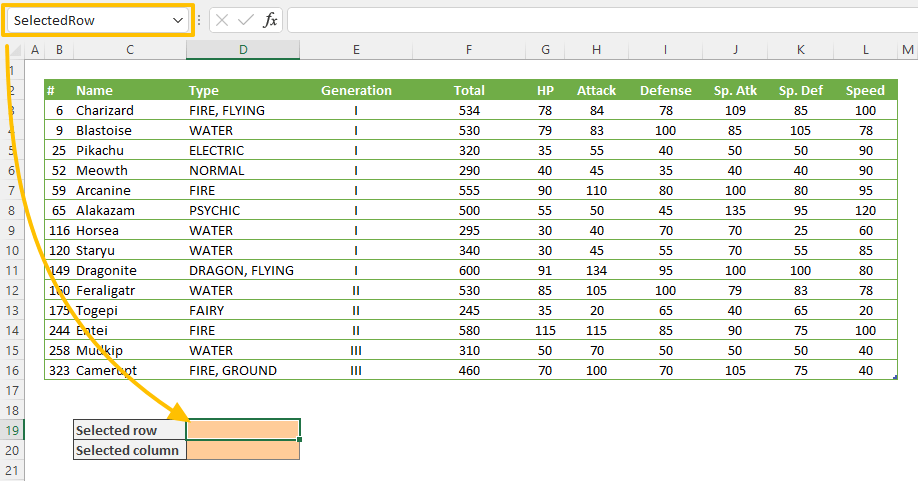
All you need to do is to select a cell and type desired name into the reference box near the formula bar. You can learn more about ways of creating named ranges in 5 Ways to Create an Excel Named Range article.
Create a named range for selected column as well, e.g., "SelectedCol".
2. VBA
Open VBA window by pressing Alt + F11 key combination. You can click Visual Basic icon under Development tab as well.

- Once VBA window is open, double click on the worksheet including the data you want to highlight. This action opens the worksheet's editor at the right side.
- Select Worksheet item in the drop down at the left. This step will add Worksheet_SelectionChange event to your editor.

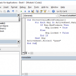
- The code under Worksheet_SelectionChange event is evaluated whenever the user selects a different cell. Either write or copy paste the following code block between "Private Sub …" and "End Sub" lines.
[SelectedRow] = Target.Row
[SelectedCol] = Target.Column


As you can figure out quickly the names between brackets refer the named ranges you created at the first step. Thus, feel free to replace them if you named your cells differently. You can learn more about how you can refer a cell or range in VBA in How to refer a range or a cell in Excel VBA.
Once the code is ready, you can close the VBA window. You can see the effect directly in your worksheet. The cells you named will show the selected cell's row and column numbers whenever you select a cell.

3. Conditional formatting
Since we know the selected cell's coordinates, it is easy to set a conditional formatting rule.
- Select the data you want to highlight.
- Open conditional formatting window by clicking Home > Styles > Conditional Formatting > New Rule.

- Select Use a formula to determine which cells to format rule.
- Type the formula which checks if the row of the cell in the data is equal the value in the "SelectedRow" cell. The reference in the ROW function should be the top-left cell of the data and a relative reference. Thus, no $ signs in the reference. Otherwise, the rule will be applied to that cell only.
=ROW(B5)=SelectedRow - Select the desired highlight color in the dialog you can reach by Format
- Click OK to save the rule.

- You can see the effect directly.

- Add another rule for the column. This time the formula should be like this:
=COLUMN(B5)=SelectedCol


That's the way of highlighting selected row and column in Excel with help of VBA.