Sure, it's easy to find the highest or smallest values in a data set. But what if you're looking for the 3rd, 10th, 20th rank in a large table, or need to do this in ascending and descending order? Luckily, Excel features a formula that does just that.
Syntax
Current use,
=RANK.EQ(the value whose rank you're looking for, array of values, sorting order)
There is an older version of this formula which should give the same result in most cases. The old formula with the same use case,
=RANK (the value whose rank you're looking for, array of values, sorting order)
Steps
- Begin by typing in =RANK.EQ( or =RANK( into a cell.
- Select or type in the range reference that includes the value (i.e. D8)
- Select or type in the range reference that includes all values (i.e. $D$8:$F$8)
- Type in 0 to set the highest value to the first place
- Type in ) and press Enter to complete the formula
Note: RANK function is an older version of the RANK.EQ function and they work exactly the same. Microsoft published a new version to include a separate function named RANK.AVG.
How
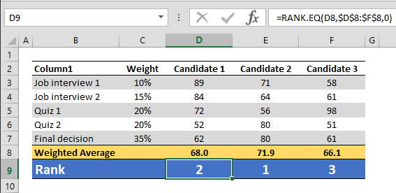
RANK.EQ function returns the mathematical placement of a number in a data set. This order can be controlled by a third optional argument. If you would like the largest number to come first, use a zero (0) as we did in our example where we found the highest score.
=RANK.EQ(D8,$D$8:$F$8,0)
Alternatively, you can set one (1) to sort in ascending order. If omitted, this value will be considered zero and the sorting will be in descending order.
The RANK function and its predecessor, RANK.EQ, both return the same values, meaning that both will give the same results for equal values. On the other hand, RANK.AVG returns the average rank of the selected value. For example, while =RANK.EQ(2,{1,2,2,2,3}) returns 2; =RANK.AVG(2,{1,2,2,2,3}) returns 3.