To return an entire row you need to use array returning functions like INDEX or OFFSET. Both of these functions can return arrays, as well as single values, which can be used in other functions like SUM, AVERAGE or even another INDEX or OFFSET. How to return an entire row article will explain you how it can be done.
Syntax
=INDEX(data without headers, MATCH(search value, headers of data, 0), 0)
=OFFSET(anchor point above headers, MATCH(search value, headers of data, 0), 1, 1, COLUMNS(any row of data or even data itself))
Steps
- Start with =INDEX( which returns the range
- Type or select the range includes data C3:E7,
- Continue with MATCH( to find the location of a desired row
- Select the range which includes the value that specifies the row H3,
- Select the range which includes the value that includes the headers B3:B7,
- Type 0), to ensure the exact match method and close MATCH
- Type 0) to specify that you want to return an entire row and close INDEX formula
How
As it is mentioned above, to return an entire column or row, you need to use array returning functions. An alternative way may be to use array functions directly. However, in most occasions they are fairly complex, unnecessary (due to existing formulas) and runs slower.
The INDEX and OFFSET are powerful functions that return a value or a range when they are combined with MATCH function which can handle the lookup process. Let's see how they work:
INDEX
The trick is to use "0" as column argument which specifies that you want to return an entire row in data instead of a single cell. The rest is how it is done with regular INDEX-MATCH. So use the MATCH function to find the location of a row:
MATCH(H3,B3:B7,0)
The INDEX function will return an array which includes values in that row.
The result: {52;80;51}
What Excel displays: 52
Please note that Excel will show only the first value of the array if you do not use them in another formula. We used the AVERAGE function to demonstrate how the array can be used.
=AVERAGE(INDEX(C3:E7,MATCH(H3,B3:B7,0),0))
The result: 70.2
OFFSET
The OFFSET function uses a similar approach as well. Instead of INDEX that you need to select the whole data range, the OFFSET requires a cell outside of the data range which can be used as an anchor point.
Another difference is the OFFSET returns an array when its optional arguments are used. These arguments basically represents the size of rows and columns to return.
Briefly; you need to specify where the row starts and how long it is. The MATCH function works the same as before to lookup the row we need and the COLUMNS function returns the row length. Of course we used "1" as column number because we only need a single row.
=AVERAGE(OFFSET(B2,MATCH(H3,B3:B7,0),1,1,COLUMNS(C2:E2)))