The power of random selection extends far beyond the basics of the RANDBETWEEN function. When dealing with non-uniform item distributions, the combination of RAND, INDEX, MATCH, and VLOOKUP functions proves invaluable for achieving precise random selection in Excel.
This guide presents two methods: the INDEX-MATCH duo and the VLOOKUP function. Both leverage the RAND function to generate random numbers, facilitating the selection of items based on predefined distribution ratios.
The INDEX-MATCH approach involves using RAND to generate a random number, MATCH to approximate its location in cumulative values, and INDEX to retrieve the corresponding item. The key lies in setting 1 as the match_type argument in MATCH, signaling the search for the largest value less than or equal to the lookup value.
Alternatively, the VLOOKUP function offers a familiar method, requiring data to be structured as a table with cumulative ratios on the left side of values. Like MATCH, VLOOKUP necessitates specifying a search type – opt for 1 or TRUE for approximate search mode.
Whether you choose the precision of INDEX-MATCH or the familiarity of VLOOKUP, mastering random selection in Excel elevates your spreadsheet skills. This guide simplifies the process, empowering you to navigate non-uniform item distributions seamlessly.
Let’s say you need to populate items randomly. You can use Excel’s RANDBETWEEN function to select a random item from a list. What if the distribution of the items is not uniform? In this article, we will show you how to select a random item by distribution in Excel.
Although Excel doesn’t have a built-in feature or function to return a value from a list, it has RAND and RANDBETWEEN functions to return a randomly generated number. In this guide, we will use RAND function to generate a random number and INDEX, MATCH, and VLOOKUP functions. The latter functions will help us to locate the randomly selected item.
This guide will show you how to select a random item by distribution in two ways:
- Using INDEX and MATCH functions
- Using VLOOKUP function
You can decide on either one based on your data structure. Let’s investigate both.
Random Selection in Excel - Sample Data
Assume that you have a list of items with distribution ratios as below.

RAND function returns a randomly generated number between 0 and 1. We can use the generated number to locate the corresponding item. First, define the slices corresponding to each item. We can create these slices with cumulative distributions.
Make sure the total distribution ratio equals 100% and start cumulative values from 0. For example, if the first item’s probability ratio is 10% the first item should be 0 and the next 10%.

As a result, we need to set formulas when RAND function returns a number between 0 and 10%, it should indicate the first item. MATCH and VLOOKUP functions can be used to handle this. They can make approximate searches to locate the closest value in the list. For example, if the search value is 7.5%, approximate search assume it is 0 in our list of 0%, 10%, 35% and 60%.
Let’s see how you can combine RAND with other functions to select a random item by distribution in Excel.
INDEX-MATCH
The first approach uses the INDEX-MATCH combination to locate and retrieve a value in a data set. The roles are clear:
- RAND returns a random number
- MATCH seeks that number in the cumulative values approximately
- INDEX returns the value by using the position number from the MATCH function
The most important thing here is using 1 for the match_type argument of the MATCH function. The 1 number indicates finding the largest value that is less than or equal to the lookup value.

Parsing Values using VLOOKUP for Random Selection in Excel
VLOOKUP is another and probably more popular way to parse values from a table. However, your data should be a table and the value should be searched in the first column. Thus, if you can or have to place cumulative ratios on the left side of your values, you can also use VLOOKUP.
Like the MATCH function, you have to indicate the search type for VLOOKUP too. Either enter 1 or TRUE to use approximate search mode.

Visit Microsoft's for further reading.