Do you have a data table where you need to pick all the highest, lowest, best, worst, or equal to 2? SUMIF and its bigger brother SUMIFS formulas can help sum cells of your choice. Follow the instructions below to learn how to sum cells in Excel.
Syntax
Step by Step
To sum cells;
- Type =SUMIF(
- Select or type range reference that you want to apply the criteria against $E$3:$E$10
- Type criteria (alternatively cell reference which contains can be used) "FL"
- Select or type range reference that includes cells to add $H$3:$H$10
- Type ) and press Enter to complete the formula
Note: When using SUMIFS, follow the steps according to the syntax of SUMIFS.
=SUMIF($E$3:$E$10,"FL",$H$3:$H$10)
=SUMIFS($H$3:$H$10,$E$3:$E$10,"FL")
How to SUM Cells in Excel?
Both functions can be used to sum cells that meet a criteria. They search a given criteria in a range; this process's result is an array of TRUE/FALSE. For example, searching FL value in $E$3:$E$10 range returns {TRUE, FALSE, FALSE, TRUE, FALSE, TRUE, TRUE, TRUE}. And then TRUE/FALSE array is matched with an array of values in the sum range, which is {$48,972, $38,828, $81,662, $44,000, $72,000, $87,633, $80,850, $80,784}. The sum of match values gives the desired result ($342,239).
However, the syntax is slightly different between formulas. Although the SUMIFS function’s criteria-based arguments come after the sum range to handle multiple criteria, using SUMIFS for single criteria is completely safe and preferable.