Using the versatile SUMIF function, see how you can create cell totals from a certain date. Creating a YTD (year-to-date) reports has never been easier.

Syntax
=SUMIFS(values to sum range, date range, >minimum date)
=SUMIF(date range, >minimum date, values to sum range)
Steps
- Type =SUMIFS(
- Select or type range reference that includes cells to add $H$3:$H$10
- Select or type range reference that includes date values you want to apply the criteria against $C$3:$C$10
- Type minimum date criteria with greater than operator ">1/1/2010"
- Type ) and press Enter to complete formula
Note: When using SUMIF, follow steps according to syntax of SUMIF.
How
Both functions can be used to add values that meet a criteria. They search a given criteria in a criteria range, this processes result is an array of TRUE/FALSE. Ability to use criteria with logical operators like greater than (>) provides the way of adding values between values.
We used ">1/1/2010" criteria to define minimum date and search is made on date range $C$3:$C$10.
=SUMIFS($H$3:$H$10,$C$3:$C$10,">1/1/2010")
=SUMIF($C$3:$C$10,">1/1/2010",$H$3:$H$10)
Alternative way to write formula is using cell references instead of static dates. For example; if your minimum date value is at cell K9, then criteria would be written as “>”&K9.
=SUMIFS($H$3:$H$10,$C$3:$C$10,">"&$K$9)
=SUMIF($C$3:$C$10,">"&$K$9,$H$3:$H$10)